
Fast Multipole Method Simulation
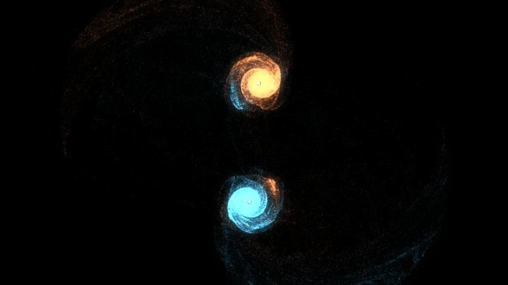
Simulate tens of thousands of bodies attracting each other by gravity, with the Fast Multipole Method (FMM): spiral galaxies, galaxy collisions, star clusters and more. See the interaction lists, measure the accuracy, and download images and videos.
This is an online Fast Multipole Method simulation: a gravitational N-body simulation where tens of thousands of bodies (stars, for example) attract each other, and the forces are computed with the Fast Multipole Method (FMM), one of the most important algorithms of the 20th century.
In a system of n bodies, every body attracts every other body, so computing the forces directly takes n·(n-1)/2 calculations on every step: 50 million for 10,000 bodies. The Barnes-Hut algorithm reduces that to about n·log(n) by treating a distant group of bodies as a single body. The FMM goes one step further: groups of bodies interact with groups of bodies, and each group is described by a multipole expansion, which captures not only its mass but also its shape. The cost drops to about n, and the forces are more accurate.
In our tests, the FMM computes the forces 2 to 3 times faster than the Barnes-Hut algorithm, while making errors 3 to 10 times smaller. At the same accuracy, it is about 7 times faster. That is enough for tens of thousands of bodies in real time, and even 100,000 bodies, directly in your browser.
Choose an initial configuration: a spiral galaxy orbiting a black hole, a collision of two galaxies, an unstable rotating disk, a cloud that collapses, merging star clusters, a ring around a black hole, or an expanding universe. Then watch gravity do the rest.
You can also see the algorithm working: draw the quadtree over the simulation, or the interaction list of one body, with the far cells that act through their expansions and the near cells computed body by body. Change the opening angle theta and the expansion order, then click Measure accuracy to compare the forces with the exact direct sum and with the Barnes-Hut algorithm.
While watching the simulation, you can pan, zoom, change the animation speed and customize the visualization: colors by speed, trails, glow and more. Move the camera by clicking and dragging your mouse on the canvas, and zoom by scrolling the mouse wheel on the canvas.
You can also record and download videos of your simulations, in webm format, and download the current animation frame as a PNG image. Everything runs directly in your browser: nothing is uploaded to a server. You are free to share the generated images and videos anywhere. Attribution is not required but appreciated.
Simulated time: 0.00
0 body pairs and 0 cell pairs per step, -× fewer than the direct sum
Examples
Below you can find some examples of gravitational simulations, and some examples that show how the Fast Multipole Method works. Click on any example to apply the configuration and start the simulation.
Spiral galaxy
A disk of 10,000 stars orbiting a supermassive black hole. The inner stars orbit faster than the outer ones, which winds the clumps of stars into spiral arms.
Galaxy collision
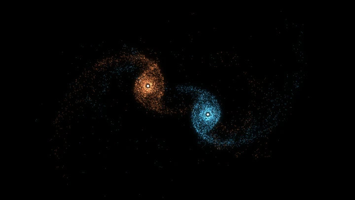
Two galaxies of 10,000 stars each pass close to each other. Their gravity pulls long tidal tails of stars out of both disks, and some stars are captured by the other galaxy. Zoom out to follow them.
Unstable rotating disk
A flat disk of stars with no black hole, where each star starts on a circular orbit. The disk is unstable: its own gravity breaks it into rings, arms and clumps, which then orbit and merge.
Cold collapse
A uniform cloud of bodies at rest falls onto itself, bounces back and settles into a dense core with a halo, a process called violent relaxation.
Merging star clusters
Eight star clusters attract each other and merge, one after the other, into a single larger cluster, like the hierarchical growth of galaxies.
Ring around a black hole
A thin ring of bodies on circular orbits. The gravity between the bodies of the ring makes small irregularities grow into clumps that orbit together.
Expanding universe
20,000 bodies spread almost uniformly fly apart slower than the escape velocity. As the expansion slows down, gravity gathers them into filaments and clumps.
A galaxy of 100,000 stars
The cost of the FMM grows in proportion to the number of bodies, so even 100,000 stars fit in your browser. The animation is slower, but a recorded video always keeps the configured framerate.
See the quadtree
A small galaxy of 1,000 bodies with the quadtree drawn on top. Each cell is split into four until it holds at most 8 bodies, so the cells are small where the bodies are dense.
The interaction list of one body
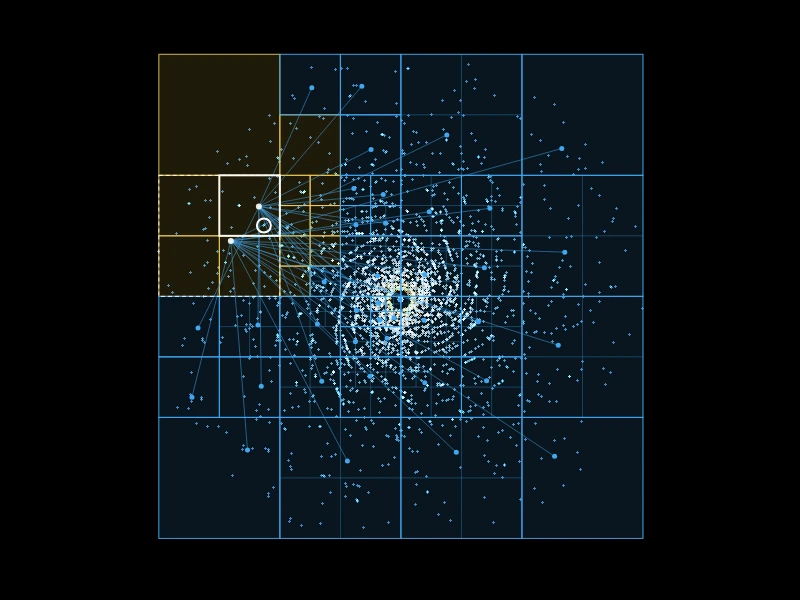
Shows how the force on one body is computed: the blue cells act through their multipole expansions on the leaf of the body or on one of its ancestors, and only the bodies of the yellow cells are computed one by one. Right click the canvas to choose another body.
Low expansion order (p = 1)
With order 1, each cell is described only by its mass, and its pull is assumed to be the same over the whole cell that receives it. In this rotating disk the forces have errors of several percent. Click "Measure accuracy" and compare with orders 4 to 8.
Exact direct sum (theta = 0)
With the opening angle equal to 0 no pair of cells is far enough, and the simulation computes every one of the n·(n-1)/2 pairs of bodies. Compare the physics time per step with the other examples.
How to create a Fast Multipole Method simulation
- Choose the initial configuration - A spiral galaxy, a collision of two galaxies, a rotating disk, a cold collapse, star clusters, a ring around a black hole or an expanding universe. Each configuration loads its recommended radius, masses and velocity factor.
- Adjust the initial conditions (optional) - Change the number of bodies, the radius, the masses, the velocity factor or the random seed.
- Adjust the physics (optional) - Change the opening angle theta, the expansion order, the number of bodies per leaf, the gravitational constant, the softening and the time step.
- Measure the accuracy (optional) - Compare the forces with the exact direct sum and with the Barnes-Hut algorithm, to see how theta and the expansion order change the speed and the errors.
- Customize the visualization (optional) - Color the bodies by speed, by galaxy or with a single color, and change their size, the brightness, the trails, the glow and the background.
- Show the quadtree (optional) - Draw all the cells of the quadtree, or the interaction list of one body: the far cells that act through their expansions and the near cells computed body by body. Right click a body on the canvas to select it.
- Watch the simulation - Use the start, pause, resume and restart buttons. Drag the mouse on the canvas to move the camera, and scroll the mouse wheel to zoom.
- Download the result - Download the current animation frame as a PNG image, or record and download a video of the simulation in webm format.
Configuration parameters
Canvas size
| Field | Description |
|---|---|
| Resolution | The canvas width and height, in pixels. You can select an option from the list of common display resolutions, or use "custom" to choose any width and height. |
| Width | The width of the animation canvas, in pixels. |
| Height | The height of the animation canvas, in pixels. |
Initial conditions
| Field | Description |
|---|---|
| Configuration | The initial arrangement of the bodies:
Choosing a configuration also loads its recommended radius, masses and velocity factor. |
| Number of bodies | The number of bodies (stars) in the simulation, including the central masses. Thanks to the Fast Multipole Method, the cost of each step grows in proportion to the number of bodies, so tens of thousands of bodies are possible, and even 100,000. The animation becomes slower with very large numbers, but a recorded video always keeps the configured framerate. |
| Radius | The radius of the galaxy, of the disk or of the cloud, in pixels. In the galaxy collision it is the radius of each galaxy, and in the star clusters it is the radius of the region where the clusters are placed. |
| Total mass of the bodies | The mass of all the bodies together, without the central masses. It is divided equally between the bodies, so changing the number of bodies does not change the overall motion: more bodies only make the image more detailed. |
| Central mass (black hole) | The mass of the body at the center of each galaxy, or at the center of the disk or the ring. Use 0 for no central mass. The central masses are drawn as white dots. |
| Number of clusters | The number of star clusters. Only used by the "star clusters" configuration. |
| Velocity factor | Multiplies the initial velocities. In the disk configurations each body starts with the speed of a circular orbit around the mass inside its radius, multiplied by this factor: 1 means circular orbits, a smaller value makes the disk contract, and a larger value makes it expand. In the star clusters, it multiplies the random velocities of the bodies inside each cluster. In the expanding universe, it is the initial expansion speed as a fraction of the escape velocity. In the cold collapse it is 0 by default, and a value greater than 0 makes the cloud rotate. |
| Random seed | The positions of the bodies are random. The same seed always generates the same initial positions, so you can reproduce a simulation. Click the dice button to try a new random seed. |
Physics
| Field | Description |
|---|---|
| Theta (opening angle) | The accuracy parameter of the FMM. Each cell of the quadtree has a radius Smaller values make more pairs of cells interact body by body, which is more accurate and slower. With theta equal to 0 no pair of cells is far enough, and the simulation computes the exact direct sum. Values between 0.5 and 0.8 are the usual compromise, and the maximum is 1, because the expansions stop converging when the cells get too close. A second criterion is always applied: a pair of cells only interacts through their expansions when the estimated error is small compared with the forces felt by their bodies on the previous step. It protects the bodies around a heavy black hole, whose pull is the strongest force of the simulation. |
| Expansion order (p) | The number of terms of the multipole and local expansions, from 1 to 8. With order 1, each cell is described only by its mass at its center of mass, and its pull is the same over the whole cell that receives it. Order 2 adds how the pull changes across the receiving cell, order 3 adds the quadrupole (how the mass is stretched), order 4 the octupole, and so on. Each order makes the forces about 2 to 3 times more accurate, but each interaction between two cells costs more. Order 4 (the default) gives average errors of a fraction of a percent. Orders 7 and 8 give average errors of a few hundredths of a percent or less, for about twice the time. |
| Bodies per leaf | The maximum number of bodies in a leaf of the quadtree: a cell with more bodies is split into four. Near leaves interact body by body, so larger leaves mean more direct pairs and fewer interactions between cells. Values between 16 and 64 are usually the fastest, and the default is 32. This option changes the speed, but almost not the accuracy. |
| Gravitational constant | The strength of gravity (the constant G of Newton's law of gravitation). Greater values make everything move faster. It multiplies all the masses, so doubling it has the same effect as doubling every mass. |
| Softening | A small distance, in pixels, added to the distance between the bodies when computing the force: the force is proportional to Without softening, two bodies passing very close to each other feel an almost infinite force and are thrown away at absurd speeds. Each body then behaves more like a small cloud of stars than like a point, which is what the bodies of a galaxy simulation really represent. The expansions of the FMM include the softening exactly, so the near and the far forces follow the same law. |
| Time step | The amount of simulated time advanced on every physics step. Smaller values make the simulation more accurate, but more steps are needed to advance the same amount of time. If bodies are thrown away from the black holes, reduce the time step or increase the softening. |
| Physics steps per frame | The number of physics steps calculated on every animation frame. The time simulated on each frame is the time step multiplied by this value and by the animation speed. |
Accuracy
| Button or value | Description |
|---|---|
| Measure accuracy | Computes the forces of the current step again, with the FMM and with the Barnes-Hut algorithm (theta 0.7), and compares them with the exact direct sum on a sample of 400 bodies. The direct sum of a sample is fast enough, while the direct sum of every body would take much longer. |
| Time | The time your computer took to build the tree and compute the forces of every body, with each method. |
| Average error and max error | The difference between the approximated force and the exact force on each body of the sample, divided by the exact force. An average error of 0.5% means that the forces are, on average, within half a percent of the exact ones. |
Visualization
| Field | Description |
|---|---|
| Color | How the bodies are colored:
|
| Body size | The diameter of each body, in pixels. A size of 1 draws each body as a single point, spread over the nearest pixels so it moves smoothly. |
| Brightness | The brightness of each body. The light of the bodies adds up, like in a long exposure photo of the sky, so the dense regions become bright and the sparse regions stay faint. Increase it when there are few bodies, and decrease it when there are many. |
| Show black holes | If enabled, the central masses are drawn as larger white dots. |
| Trails | How much of the previous frame remains visible, from 0 (no trails) to 0.99 (very long trails). The trails are drawn on the canvas, so moving or zooming the camera also leaves a trail. |
| Glow | If enabled, a blurred copy of the bodies is added over the image, which gives the galaxies a soft glow. |
| Glow radius | The radius of the blur of the glow, in pixels. |
| Glow intensity | The strength of the glow, from 0 to 2. |
Quadtree
| Field | Description |
|---|---|
| Show quadtree | Hidden: only the bodies are drawn. All the cells: draws the leaves of the quadtree built on the current step. Each cell with more bodies than the "bodies per leaf" option is split into four smaller cells, so the cells are small where the bodies are dense. A cell whose bodies are all in the same quarter shrinks to that quarter, so empty regions have no cells. Interaction list of the selected body: shows how the force on the selected body (marked with a white circle) is computed. The white square is the leaf that contains the body, and the dashed white squares are its ancestors that received expansions. The blue cells are the far cells: the multipole expansion of each one was converted into a local expansion of the leaf or of an ancestor, and the lines link the centers of mass of the two cells of each conversion. The yellow cells are the near cells, whose bodies were computed one by one. Right click a body on the canvas to select it. |
| Quadtree color | The color of the cells of the quadtree, and of the far cells of the interaction list. |
| Select a random body | Selects another body at random, and shows its interaction list. |
Coordinates
| Field | Description |
|---|---|
| Origin | The coordinates origin (0,0), which is where the center of the galaxy is placed. It can be "top left" or "center". |
| Offset x | The "x" coordinate offset, in pixels. It determines the horizontal position of the "camera". Adjusting this offset lets you shift the view or "move" the camera. |
| Offset y | The "y" coordinate offset, in pixels. It determines the vertical position of the "camera". |
Zoom
| Field | Description |
|---|---|
| Zoom | Changing this parameter allows you to "zoom in" or "zoom out". You can also zoom by scrolling the mouse wheel on the canvas. The bodies keep their size in pixels, only the distances between them change. |
Background
| Field | Description |
|---|---|
| Transparent background | If this option is checked, the animation has a transparent background. |
| Background color | The background color, in hexadecimal value. For example, use #000000 for a black background. |
Animation speed
| Field | Description |
|---|---|
| Animation speed | The speed of the animation. Values greater than 1 mean the animation plays in "fast motion", and values smaller than 1 mean it plays in "slow motion". It changes the number of physics steps per frame, so the accuracy of the simulation stays the same. |
Animation control
| Button or value | Description |
|---|---|
| Start | Start the simulation. |
| Restart | Restart the simulation from the initial conditions. |
| Pause | Pause the simulation. |
| Resume | Resume the simulation. |
| Stop | Stop the simulation. |
| Quadtree cells | The number of cells of the quadtree built on the last step, the number of leaves, and the depth (the number of times the root cell was split to reach the smallest cell). |
| Body pairs per step (direct) | The number of pairs of near bodies whose force was computed directly on the last step. Each pair is computed once for both bodies. |
| Cell pairs per step (M2L) | The number of pairs of far cells that interacted through their expansions (multipole-to-local conversions) on the last step. Each one replaces the forces between all the bodies of the two cells. |
| Direct sum | The number of pairs of bodies of the exact direct sum, n·(n-1)/2, and how many times more pairs it computes than the FMM. |
| Physics time per step | The time your computer took to build the quadtree, compute the expansions and the forces, and move the bodies, on each step. |
| Download current animation frame | Download the current animation frame (in PNG format). |
| Reset all the options | Restore every option to its default value and restart the simulation. |
Generate and download video
Instead of only watching the simulations online, you can also record and download videos of your simulations. The simulation videos are generated using the webm extension.
| Field | Description |
|---|---|
| Framerate | The amount of frames per second that you want the video to have. |
| Automatically stop after... | If enabled, the video recording stops automatically after the configured time (in seconds) or after the configured amount of frames. |
How the Fast Multipole Method works
Newton's law of gravitation says that every body attracts every other body with a force proportional to the product of their masses and inversely proportional to the square of the distance between them. To move n bodies one step forward, a simulation needs the total force on each body, and the direct way to get it computes the force of each of the n·(n-1)/2 pairs of bodies. Doubling the number of bodies makes each step four times slower.
The Fast Multipole Method was introduced by Leslie Greengard and Vladimir Rokhlin in 1987, and was later listed among the top 10 algorithms of the 20th century. Like the Barnes-Hut algorithm, it organizes the bodies in a tree, so that distant groups of bodies can be handled together. On every step, the simulation:
- Builds a quadtree - A square that contains every body is the root of the tree. Any square with more bodies than the "bodies per leaf" option is split into four smaller squares, and so on.
- Computes the multipole expansion of each cell (upward pass) - Each leaf summarizes its bodies around their center of mass: the total mass, then the quadrupole (how the mass is stretched), the octupole and the higher terms up to the expansion order. Each parent cell combines the expansions of its children, shifted to its own center of mass, without looking at the bodies again.
- Finds the interactions between cells (dual tree traversal) - Starting from the pair (root, root), the simulation looks at pairs of cells. When two cells are far apart compared to their sizes, the multipole expansion of each one is converted into a local expansion around the center of the other one: a Taylor series that gives the pull of the far cell anywhere inside the near one. This multipole-to-local conversion (M2L) serves all the bodies of both cells at once. Pairs of near, small cells are computed body by body, and the other pairs are split into the pairs of their children.
- Passes the local expansions down the tree (downward pass) - The local expansion of each cell is shifted to the center of each child and added to the child's own expansion. At the leaves, it is evaluated at each body, which gives the pull of every far body at once.
- Moves the bodies - The velocities and the positions are updated with the leapfrog integrator (kick-drift-kick), which is time-reversible and keeps the energy of the orbits stable over long simulations.
Because each cell interacts with a limited number of other cells, whatever the number of bodies, the total cost of a step grows in proportion to n, instead of n·log(n) for the Barnes-Hut algorithm. And because every interaction is computed once for both cells or both bodies, the forces obey Newton's third law exactly: the total momentum of the system is conserved, up to rounding errors.
This tool uses the Cartesian form of the FMM described by Walter Dehnen for his "falcON" code, where the expansions are Taylor series of the softened potential 1 / sqrt(d² + softening²). The classic two-dimensional FMM of Greengard and Rokhlin uses complex numbers, but it describes the logarithmic potential of a truly two-dimensional gravity, where the force decreases as 1 / d. This tool keeps the inverse square law of the real universe, like the Barnes-Hut simulation, so the two tools simulate exactly the same physics and can be compared directly.
The bodies move on a plane: real galaxies are three dimensional, but their disks are thin, so a 2D simulation already reproduces many of their features: spiral arms, bars, tidal tails and mergers.
Frequently Asked Questions (FAQ)
What is the Fast Multipole Method?It is an algorithm that computes the interactions between many particles (gravitational, electrostatic, and others) in a time proportional to the number of particles, instead of the square of that number. It groups the particles in the cells of a tree, describes each group with a multipole expansion, and lets groups interact with groups. It is used in astrophysics, molecular dynamics, acoustics and electromagnetism.
Is the FMM faster than the Barnes-Hut algorithm?Yes, but not by orders of magnitude at the sizes that run in a browser. In our tests with the default options, the FMM computed the forces 2 to 3 times faster than the Barnes-Hut algorithm with theta 0.7, while its average errors were 3 to 10 times smaller: for 20,000 bodies, about 12 to 16 ms per step instead of 30 to 45 ms. To make the Barnes-Hut algorithm as accurate as the FMM, theta must be lowered to about 0.3, and then the FMM is about 7 times faster. Click "Measure accuracy" to compare both methods on your own computer.
Why is the FMM faster, if log(n) is so small?For 20,000 bodies, log(n) is small, so the difference between n and n·log(n) alone explains little. Most of the gain comes from elsewhere: a single cell-to-cell interaction replaces the interactions of all the bodies of both cells, each interaction is computed once for both sides, and the higher order expansions reach a given accuracy with far fewer interactions than the single center of mass of the Barnes-Hut algorithm.
It is a description of a group of masses as seen from far away, term by term. The first term (the monopole) is the total mass at the center of mass. Around the center of mass the dipole term is zero, and the next terms, the quadrupole, the octupole and so on, describe how the mass is stretched or bent. The farther away you are, the less the higher terms matter, so a few terms are enough to compute the pull of a distant group very accurately.
What is the N-body problem?The N-body problem is the problem of predicting the motion of a group of bodies that interact through gravity. With two bodies the orbits are simple ellipses, but with three or more bodies there is no general formula, and the motion must be computed numerically, step by step. See also the Three-Body Problem Simulation.
Why is the total momentum conserved exactly?Because every interaction is mutual: the force of cell A on cell B is computed together with the force of B on A, with the same numbers, so they cancel exactly when added up. In the Barnes-Hut algorithm each body computes its own force, and the force of a body on a group is not exactly the opposite of the force of the group on the body, so the system can slowly drift.
How many bodies can I simulate?There is no hard limit. A typical computer runs 10,000 to 20,000 bodies in real time, and 100,000 bodies at a lower framerate. If the animation becomes slow, record a video instead, because the video always keeps the configured framerate.
Which units are used?The distances are in pixels and the time is in arbitrary simulation units. The masses and the gravitational constant have no units either: only their product matters for the motion.
Are my simulations uploaded to a server?No. Everything runs in your browser, on the HTML canvas. Nothing is uploaded, and the images and videos you download are generated on your own computer.
Can I use the generated images and videos?Yes. You are free to use and share the generated images and videos on YouTube, TikTok, or any other social media or website. Attribution is not required but appreciated.
Related tools