Turing machines
What a Turing machine is, how it works, and how its many types and variations are classified, explained from the beginning.
In 1936, long before the first electronic computer was built, a young English mathematician called Alan Turing imagined a very simple machine: a strip of paper, a head that reads and writes one symbol at a time, and a short list of rules. Today we call it a Turing machine.
It looks almost too simple to be useful, and yet it can do everything that any computer can do: your phone, your laptop and the largest supercomputers in the world can't solve a single problem that a Turing machine can't. That is why, 90 years later, it is still the standard way to answer the question "what can a computer do, and what can it never do?".
This article explains, without assuming any knowledge of computer science, what a Turing machine is, how it runs, what it can and can't do, and the many types of Turing machines that people have invented since, with diagrams that show how they are classified. You can also run real Turing machines in your browser with our Turing Machine simulator.
Contents
- What is a Turing machine?
- The parts of a Turing machine
- How a Turing machine runs
- An example: adding 1 to a binary number
- Try it: run a Turing machine step by step
- Halting, running forever, and the halting problem
- The universal Turing machine
- The Church-Turing thesis and Turing completeness
- The formal definition
- Types and variations of Turing machines
- How Turing machines are classified
- Frequently asked questions
What is a Turing machine?
A Turing machine is not a real machine made of metal and wires. It is an imaginary machine, a mathematical model of what it means to compute something by following rules. Turing called it an "automatic machine"; the name "Turing machine" was given to it a year later by the American logician Alonzo Church.
In 1936 the word "computer" meant a person: someone, often in a bank or in an observatory, whose job was to do long calculations with pencil and paper. Turing asked what such a person really does, step by step, and stripped it down to the bare minimum:
- The paper becomes a long strip divided into squares, with one symbol in each square.
- The person looks at only one square at a time, and can change what is written there.
- Then they move their attention one square to the left or to the right.
- What they do depends only on the symbol they see and on their "state of mind" (what they were doing, like "I'm carrying a 1"), and there are only finitely many states of mind.
Turing argued that any calculation a person can do by following precise instructions can be broken down into these tiny steps. He wrote all this in a famous paper, On Computable Numbers, with an Application to the Entscheidungsproblem, where he used his machine to answer one of the big open questions of mathematics: is there a mechanical method that can decide whether any mathematical statement is true? His answer was no, and we will see why in the section about the halting problem.
The parts of a Turing machine
Every Turing machine has the same four parts. Only the rules change from one machine to another.
- The tape - A strip of cells that goes on forever in both directions. Each cell holds one symbol from a small fixed set, the alphabet, like 0 and 1. Cells that were never written hold a special blank symbol, written here as
_. The tape is the machine's memory, and since it is endless, the machine never runs out of memory. - The head - It sits on one cell at a time. At each step it reads the symbol in that cell, can replace it with another symbol, and then moves one cell to the left or to the right.
- The state - The machine is always in one of a finite number of states, like "right", "carry" and "done". The state is a tiny memory that says what the machine is in the middle of doing. One state is the start state, and some states are halting states, where the machine stops.
- The rules - Also called the transition table or the program. For each combination of state and symbol read, a rule says three things: which symbol to write, which way to move, and which state to go to next.
That's all. There is no addition, no comparison, no "if" or "loop" built into the machine. Everything a Turing machine does, it does by combining these tiny steps.
How a Turing machine runs
Before it starts, the input is written on the tape (all the other cells are blank), the head is placed on the first symbol of the input, and the machine is put in its start state. Then it repeats the same cycle again and again:
- Read the symbol under the head.
- Find the rule for the current state and the symbol just read.
- Write the symbol the rule says (it can be the same one, which changes nothing).
- Move the head one cell left or right.
- Change to the next state the rule says (it can be the same state).
The machine stops, or halts, when it reaches a halting state, or when there is no rule for the current state and symbol. Whatever is written on the tape at that moment is the output.
Notice that the machine never "thinks" or chooses: at each step there is exactly one rule that applies, so the same input always produces the same run. That is why this kind of machine is called deterministic.
An example: adding 1 to a binary number
Computers store numbers in binary, using only the digits 0 and 1. For example, 1011 in binary is 8 + 0 + 2 + 1 = 11. To add 1 to a binary number you do the same as with ordinary numbers: start at the last digit, and while it is 1 turn it into 0 and carry 1 to the left, until you find a 0 (or the end of the number), which becomes 1. So 1011 + 1 = 1100, that is, 11 + 1 = 12.
Here is a Turing machine that does exactly that, with three states:
- right - walk to the right over the digits until the blank after the number, then step back onto the last digit.
- carry - while reading 1, write 0 and keep going left; when reading 0 (or a blank, if all the digits were 1), write 1 and finish.
- done - the halting state.
| State | Reads | Writes | Moves | Next state |
|---|---|---|---|---|
| right | 0 | 0 | Right | right |
| right | 1 | 1 | Right | right |
| right | _ | _ | Left | carry |
| carry | 1 | 0 | Left | carry |
| carry | 0 | 1 | Left | done |
| carry | _ | 1 | Left | done |
The same rules are often drawn as a state diagram: each state is a circle, and each rule is an arrow from one state to another, labeled with "symbol read → symbol written, move".
Try it: run a Turing machine step by step
Click Step to run one rule at a time, or Run to let the machine go on its own. The highlighted row of the table is the rule that will be used next. You can type another binary number, or switch to the 2-state busy beaver, a famous little machine that starts on a tape full of zeros.
_
_
1
0
1
1
_
_
State: right
Steps: 0
In state "right" the head reads "1". The rule says: write "1", move right, go to state "right".
Rules
| State | Reads | Writes | Moves | Next |
|---|---|---|---|---|
| right | 0 | 0 | R | right |
| right | 1 | 1 | R | right |
| right | _ | _ | L | carry |
| carry | 1 | 0 | L | carry |
| carry | 0 | 1 | L | done |
| carry | _ | 1 | L | done |
History: one row per step
0__1011__right
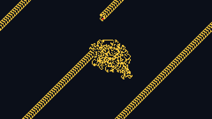
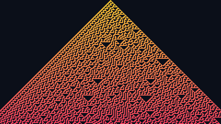
The history on the right is a space-time diagram: the tape is drawn again after every step, one row below the other, so the whole computation can be seen at once. Our Turing Machine simulator draws the same kind of picture for machines that run for thousands or millions of steps, one pixel per cell, and the result can be surprisingly beautiful.
Halting, running forever, and the halting problem
A Turing machine doesn't have to stop. Started on some input, it can do one of two things:
- Halt after a finite number of steps. The tape then holds the answer. Machines that answer yes-or-no questions often have two halting states, accept and reject.
- Run forever. Sometimes it is easy to see, like a machine stuck going back and forth between two cells. Sometimes it is extremely hard to tell whether the machine will stop one day or not.
Turing asked: could there be a Turing machine that looks at the rules of any machine and its input, and always tells correctly, in a finite time, whether that machine will halt? This is the halting problem, and Turing proved that no such machine can exist. The idea of the proof fits in a few lines:
- Suppose there is a machine H that always answers correctly "halts" or "runs forever" about any machine and input.
- Build a contrarian machine D that takes the rules of a machine M, asks H what M does when given its own rules as input, and then does the opposite: if H says "halts", D runs forever; if H says "runs forever", D halts.
- Now give D its own rules. If D halts, then H said "runs forever", so H was wrong. If D runs forever, then H said "halts", so H was wrong again.
- Either way H is wrong about D, so a machine like H can't exist.
This was a shock: it showed that there are perfectly well-defined questions that no computer will ever be able to answer, however fast it is and however long it runs. Problems like this are called undecidable.
The halting problem is behind a famous game, the busy beaver: among all the machines with a given number of states that start on an empty tape and eventually halt, which one runs the longest? With 2 states the champion halts after 6 steps (it's the one in the demo above), with 3 states after 21 steps, with 4 states after 107 steps, and with 5 states after 47,176,870 steps, a value that was only proven in 2024 by an online collaboration of volunteers, the Busy Beaver Challenge. For 6 states nobody knows the answer, but some machines are known to halt after more than 101010⋰ steps, a tower of fifteen 10s stacked as exponents. You can run the busy beavers in our Turing Machine simulator.
The universal Turing machine
Each Turing machine has its own fixed rules, so it seems that we need a different machine for every task: one to add numbers, one to sort a list, one to play chess. Turing's most important discovery, in the same 1936 paper, is that this is not necessary.
The rules of any Turing machine are just a finite table, so they can be written on a tape as a sequence of symbols. Turing showed how to build one special machine, the universal Turing machine, that reads such a description of another machine M, followed by an input, and then imitates M step by step, giving exactly the same result as M would.
This is the idea of the stored-program computer, and it's exactly what your computer does: it is one fixed piece of hardware, and the programs it runs are just data stored in its memory. John von Neumann, who described the design used by almost all computers since the 1940s, knew Turing's work well.
The Church-Turing thesis and Turing completeness
In the same year as Turing, Alonzo Church described a completely different way of computing, the lambda calculus, based on functions instead of machines. Other people proposed other models: recursive functions, Post's rewriting systems, and later register machines and programming languages. Remarkably, all of them turned out to be able to compute exactly the same things as Turing machines: each one can imitate the others.
This led to the Church-Turing thesis: anything that can be computed by following a step-by-step procedure (an algorithm) can be computed by a Turing machine. It isn't a theorem that can be proven, because "following a procedure" is an informal idea, but in 90 years no one has found a reasonable counterexample.
A system that can imitate any Turing machine is called Turing complete. Almost every programming language is Turing complete, and so are some systems that were never meant to compute anything:
- Conway's Game of Life, a grid of cells that live or die according to their neighbors. People have built working Turing machines and even whole computers out of its patterns.
- Rule 110, an elementary cellular automaton where each cell only looks at itself and its two neighbors, was proven Turing complete by Matthew Cook.
- Spreadsheet formulas, some board and card games, and the redstone circuits of some video games.
The Game of Life and Rule 110 are cellular automata, grids of cells that all follow the same simple rule. Our article about cellular automata explains how they work.
Strictly speaking, a real computer is not quite a Turing machine, because its memory is finite, while the tape of a Turing machine never ends. But its memory is so large that, for most purposes, the Turing machine is a very good model of it.
The formal definition
In books, a Turing machine is usually defined as a list of seven things, a "7-tuple" M = (Q, Γ, b, Σ, δ, q0, F). It looks scary, but it is just the parts we have already seen, with names. The last column shows them for our binary machine.
| Symbol | Name | Meaning | In the example |
|---|---|---|---|
| Q | States | The finite set of states. | {right, carry, done} |
| Γ | Tape alphabet | The finite set of symbols that can be on the tape. | {0, 1, _} |
| b | Blank symbol | The symbol of the cells that were never written. It belongs to Γ. | _ |
| Σ | Input alphabet | The symbols allowed in the input, a part of Γ without the blank. | {0, 1} |
| δ | Transition function | The rules: for a state that is not halting and a symbol, it gives the symbol to write, the move (L or R) and the next state. | The six rules of the table above, like δ(carry, 1) = (0, L, carry) |
| q0 | Start state | The state the machine is in at the beginning. | right |
| F | Halting states | The states where the machine stops (sometimes split into accepting and rejecting). | {done} |
A snapshot of the machine at one moment, made of the content of the tape, the position of the head and the current state, is called a configuration. A run of the machine is a sequence of configurations, each one obtained from the previous one by applying one rule.
Types and variations of Turing machines
Since 1936, people have invented many variations of the Turing machine: with more tapes, with a 2D grid instead of a tape, with the power to guess, to flip coins, or to use quantum physics. A surprising fact is that almost none of these changes adds any computing power. A plain one-tape machine can imitate all of them: it may need many more steps, but it gets the same answers. Only two kinds of change really matter: taking something essential away, which makes the machine weaker, or adding something impossible to build, which makes it stronger (in theory).
The diagram below groups the variations by what they change. Click a group to jump to its explanation.
Standard Turing machine
one infinite tape, one head, one rule for each state and symbol
Change the tape
- Tape infinite in one direction onlySame power
- Tape with several tracksSame power
- Several tapes (multi-tape)Same power
- 2D tape (turmites)Same power
Change the head
- Several headsSame power
- Head that can stay putSame power
Change the symbols and states
- Only 2 symbolsSame power
- Only 2 statesSame power
- Non-erasing (Wang B-machine)Same power
Change how the next step is chosen
- NondeterministicSame power
- ProbabilisticSame power
- QuantumSame power
- AlternatingSame power
- ReversibleSame power
Restrict it
- Linear bounded automatonLess power
- Tape used as a stack (pushdown automaton)Less power
- Read-only tape (finite automaton)Less power
Give it superpowers
- Oracle machineMore power (theory only)
- Infinite time Turing machineMore power (theory only)
Variations of the tape
- Tape infinite in one direction only (semi-infinite tape) - The tape has a first cell and goes on forever only to the right. Many textbooks use this version. It has the same power: the machine can fold the two halves of an infinite tape into one, using even cells for one half and odd cells for the other.
- Tape with several tracks - Each cell is divided into several rows, like a spreadsheet with a few lines, and the head reads all of them at once. This is really the same as a single tape with a bigger alphabet, where each symbol is a combination like (1, 0, _).
- Several tapes (multi-tape Turing machine) - The machine has, say, three tapes, each with its own head that moves independently, and each rule depends on the three symbols read. It's much more convenient (one tape for the input, one for scratch work, one for the output) and can be much faster, but a one-tape machine can imitate it: what the multi-tape machine does in t steps takes the one-tape machine about t² steps.
- 2D tape - The tape is replaced by an infinite grid, like a sheet of squared paper, and the head moves up, down, left and right. These machines are called turmites, and the simplest of them is the famous Langton's ant. They draw amazing patterns, but they can't compute anything a normal Turing machine can't. Try them in our Turmite simulator.
Variations of the head
- Several heads on the same tape - Each head reads and moves on its own. Again convenient, again the same power.
- Head that can stay put - Besides left and right, a rule can say "stay". A normal machine imitates it by moving right and then left again.
- Head that jumps several cells at once, or moves to any position directly (this is close to how the memory of a real computer works, called random access). Same power, only faster.
Variations of the symbols and states
- Only 2 symbols - Any machine can be converted into one that only uses blank and 1 (or 0 and 1), by writing each symbol as a short code of several cells, the same way a computer stores letters as groups of bits. The Post-Turing machine, inspired by a model that Emil Post described in 1936, the same year as Turing, is a version like this, with instructions closer to a simple program.
- Only 2 states - In 1956, Claude Shannon, the founder of information theory, showed something surprising: any machine can be converted into one with just 2 states, if it is allowed more symbols. States and symbols can be traded for each other.
- Non-erasing machines - In 1957 Hao Wang described a machine that can write marks but can never erase them (the Wang B-machine). Even this machine has the same power, because it can always copy its work to a fresh part of the tape instead of erasing.
Variations of how the next step is chosen
This group is the most important for understanding modern computer science. These machines all compute the same things as the standard machine, but some of them may be much faster for some problems, and the question of how much faster is one of the biggest open questions in mathematics.
- Deterministic Turing machine - The standard machine: for each state and symbol there is exactly one rule, so there is only one possible run.
- Nondeterministic Turing machine - For the same state and symbol there can be several rules, and the machine can follow any of them. You can imagine that at every choice the machine splits into copies that try all the options at once, or that it always makes a lucky guess. It answers "yes" if at least one of the paths answers "yes". A deterministic machine can imitate it by trying all the paths one after another, but that can take exponentially longer.
- Probabilistic Turing machine - At some steps the machine flips a coin to choose between two rules. It's allowed to be wrong sometimes, as long as it's right most of the time (for example, with probability at least 2/3; repeating the run many times then makes errors as rare as we want). Many fast algorithms used in practice, like the tests that check whether a huge number is prime, are probabilistic.
- Quantum Turing machine - Described by David Deutsch in 1985, it follows the laws of quantum physics: it can be in a superposition of many configurations at once, which can interfere with each other like waves. It is the theoretical model of quantum computers. It can't compute anything a normal machine can't, but for some problems, like breaking large numbers into their prime factors (Shor's algorithm), it is believed to be exponentially faster.
- Alternating Turing machine - A generalization of the nondeterministic machine with two kinds of states: in "there exists" states it accepts if at least one path accepts, and in "for all" states it accepts only if all paths accept. It's like a game between two players, where one tries to prove the answer is yes and the other tries to prove it's no, and it's useful to study games like chess or Go on boards of any size.
- Reversible Turing machine - A machine where every configuration has at most one possible previous configuration, so the run can always be played backwards. In 1973 Charles Bennett showed that any computation can be done reversibly. This matters for physics: erasing information always costs a tiny amount of energy (Landauer's principle), and reversible computing avoids erasing.
Weaker machines: taking something away
If we take away something essential from a Turing machine, it becomes a weaker kind of machine, called an automaton. These machines are very important in practice, because they are simpler, faster and, unlike Turing machines, we can always predict what they will do.
- Linear bounded automaton - The head can't leave the part of the tape where the input was written. The machine can still write and erase, but its memory is limited by the size of the input.
- Pushdown automaton - The machine reads the input once, from left to right, and has extra memory that works like a stack of plates: it can only put a symbol on the top or take the top one off. This is enough to check that parentheses are balanced, and it's how programming languages are read by compilers. Curiously, with two stacks it becomes as powerful as a Turing machine again, because two stacks together work like a tape, one holding everything left of the head and the other everything to the right.
- Finite automaton (finite state machine) - The machine can only read the tape, without writing, so its only memory is its current state. Traffic lights, vending machines and the search patterns of text editors (regular expressions) work like this.
More powerful than a Turing machine (in theory)
Machines that can compute more than a Turing machine are called hypercomputers. They are useful thought experiments for mathematicians, but nobody knows how to build one, and most scientists believe it is impossible.
- Oracle machine - Introduced by Turing himself in 1939: a Turing machine connected to a black box, the oracle, that instantly answers one kind of question, even an undecidable one like the halting problem. It is used to compare how hard different unsolvable problems are. Even an oracle machine has its own halting problem that it can't solve, so there is an endless ladder of harder and harder problems.
- Infinite time Turing machine - A machine allowed to run for infinitely many steps and then keep going, defined by Joel David Hamkins and Andy Lewis in 2000. It can solve the halting problem of ordinary Turing machines simply by running them "until the end of time".
Famous individual machines
- Universal Turing machines - Machines that can imitate any other machine, as explained above. People compete to find the smallest ones, counted in states and symbols. For example, Yurii Rogozhin found a universal machine with only 4 states and 6 symbols. In 2007, Alex Smith proved that a machine with just 2 states and 3 symbols, proposed by Stephen Wolfram, is universal, but in a weaker sense, because it needs a tape that is already filled with an infinite, non-repeating pattern at the start.
- Busy beavers - The machines that run for the longest time before halting, among all the machines of their size, as described above.
How Turing machines are classified
There are several ways to classify Turing machines and their relatives, depending on the question we ask: what problems can it solve at all, how fast can it solve them, and how does it behave when it runs?
By computing power: what problems can it solve?
Ordering the machines by the problems they can solve gives a set of nested boxes: every machine can solve all the problems of the boxes inside it, and more. For the inner four levels, this is the Chomsky hierarchy, named after the linguist Noam Chomsky, who classified the grammars of languages in the same way in 1956.
Hypercomputers (only in theory)
Oracle machines, infinite time Turing machines. Can solve the halting problem of ordinary Turing machines.
Turing machines and every variation with the same power
Semi-decidable problems: when the answer is "yes", the machine will eventually say so, but when it's "no" it may run forever. Example: "does this program ever stop?".
Turing machines that always halt (deciders)
Decidable problems: the machine always gives an answer, "yes" or "no". Everything a computer can always solve, given enough time and memory.
Linear bounded automata
Memory limited to the size of the input. Example: are there as many a's as b's and as c's in "aaabbbccc"?
Pushdown automata
Memory as a stack. Example: are the parentheses in "(()(()))" balanced?
Finite automata
No memory except the current state. Example: does this binary number end in 0 (is it even)?
Note that "Turing machines that always halt" are not a different design, but ordinary Turing machines with a guarantee about their behavior. The gap between the two boxes is exactly where the undecidable problems live, like the halting problem.
By speed: how much time and memory does it need?
The variations with the same power can still be very different in speed. Complexity theory classifies problems by the time or memory a given kind of machine needs to solve them, as the input gets bigger. "Polynomial time" means the number of steps grows like a power of the input size, like n² or n³, which is considered fast; "exponential time" means it grows like 2n, which quickly becomes hopeless. Each kind of machine defines its own class of problems:
| Class | Machine | Problems it contains |
|---|---|---|
| P | Deterministic Turing machine, in polynomial time | Problems that can be solved quickly, like sorting a list or finding the shortest route on a map. |
| NP | Nondeterministic Turing machine, in polynomial time | Problems whose solutions can be checked quickly, even if finding them seems hard, like solving a sudoku of any size: filling it in may take forever, but checking a filled grid is easy. |
| BPP | Probabilistic Turing machine, in polynomial time, right most of the time | Problems that can be solved quickly by flipping coins. Many researchers believe that BPP is actually equal to P. |
| BQP | Quantum Turing machine, in polynomial time, right most of the time | Problems that a quantum computer can solve quickly, like factoring large numbers. |
| PSPACE | Deterministic Turing machine with polynomial memory (any time). The same as AP, the alternating machine in polynomial time | Includes finding the winner of many two-player games played on boards of any size. |
| EXPTIME | Deterministic Turing machine, in exponential time | Includes finding the winner in chess and Go played on boards of any size. It's known that P is smaller than EXPTIME. |
Whether P equals NP, that is, whether every problem whose solution is easy to check is also easy to solve, is the famous P versus NP problem, one of the seven Millennium Prize Problems, with a prize of one million dollars for its solution. In terms of machines, it asks: is a nondeterministic Turing machine really faster than a deterministic one?
The table below shows how expensive it is for a standard one-tape machine to imitate each variation. If a machine takes t steps, the imitation takes about:
| Variation | Steps needed by a one-tape machine to imitate t steps |
|---|---|
| Tape with several tracks, more symbols | t: no slowdown at all |
| Tape infinite in both directions, head that can stay put | A small multiple of t |
| Several tapes | About t² (quadratic) |
| Several heads, 2D tape, random access memory | A power of t (polynomial) |
| Nondeterministic, alternating | Exponential, like 2t, as far as anyone knows |
| Probabilistic, quantum | Exponential in general, as far as anyone has proven (by trying every coin flip, or every branch of the superposition) |
| Oracle machine, infinite time Turing machine | Impossible: no Turing machine can imitate them |
By behavior: what does it do when it runs?
A third way to classify machines is to look at what they actually do. The volunteers of the Busy Beaver Challenge, who had to examine tens of millions of machines with 5 states to find the champion, sorted the machines that run forever into families with typical behaviors, so that each family can be recognized and proven to never halt. The space-time diagrams below show four of them, each starting on an empty tape (time goes down, and the yellow cell is the head):
Halts
1RB1RZ_1LB0RC_1LC1LAThe 3-state busy beaver stops after 21 steps. The red cell is where it halts.
Cycler
1RB0RC_1LC0RA_0LC1LAAfter a few steps, the whole tape repeats every 14 steps, forever, without moving away.
Translated cycler
1RB1LA_1LA0RAThe same short dance repeats forever, but each time one cell further to the right.
Bouncer
1LB1RA_1RA1LBThe head bounces between the two ends of a block that grows by one cell at each visit.
Other families include counters, which count in binary on the tape forever, like our example machine adding 1 again and again, and machines whose behavior looks chaotic, with no visible pattern. The machines are written in the compact notation of the busy beaver community: one group per state (A, B, C), and for each symbol read (0, then 1) what to write, where to move and the next state, with Z as the halting state. You can paste them into our Turing Machine simulator to watch them run for longer.
Frequently asked questions
Is my computer a Turing machine?
Almost. A computer can do everything a Turing machine can do, as long as it doesn't run out of memory, and a Turing machine can imitate everything a computer does. The only difference is that the tape of a Turing machine is infinite, while the memory of a computer is finite.
Has anyone built a real Turing machine?
Turing machines were never meant to be built: they are far too slow to be practical. But people have built physical ones for fun and for museums, with a strip of tape or paper and a moving head, and some have even been built out of LEGO bricks or wooden parts. The easiest way to see one running is a simulator like our Turing Machine tool.
What does "Turing complete" mean?
A programming language or a system is Turing complete if it can imitate any Turing machine, which means it can compute everything that is computable, given enough time and memory. Most programming languages are Turing complete, and so are some unexpected things, like the Game of Life.
Is a Turing machine the same as the Turing test?
No. Both were invented by Alan Turing, but the Turing test, from 1950, is a test of whether a machine can hold a conversation that can't be told apart from a human's. The Turing machine, from 1936, is a model of computation.
Are Turing patterns related to Turing machines?
Only through their author. Turing patterns, the spots and stripes of animal skins, come from a paper about chemistry and biology that Turing wrote in 1952. You can create them with our Turing Pattern Generator.
Are quantum computers more powerful than Turing machines?
Not in what they can compute: a normal Turing machine can imitate a quantum computer, only exponentially slower as far as anyone knows. Quantum computers may be much faster for some problems, but they can't solve undecidable problems like the halting problem.
Further reading
- Turing Machines, in the Stanford Encyclopedia of Philosophy.
- Turing machine and Turing machine equivalents, on Wikipedia.
- The Busy Beaver Challenge, the collaboration that proved the value of the 5-state busy beaver.
Related tools