
Cellular automata
What a cellular automaton is, how simple rules create complex patterns, and how the many kinds of cellular automata are classified, explained from the beginning.
Take a sheet of squared paper and color a few squares. Now follow one simple rule, the same for every square: look at the squares around it, and decide whether it will be colored in the next drawing. Repeat, again and again. This is a cellular automaton, and it is one of the most surprising ideas in science: rules so simple that a child can follow them can produce patterns that move, grow, reproduce, look alive, and can even compute anything a computer can.
This article explains, without assuming any knowledge of mathematics or programming, what a cellular automaton is, how the famous elementary cellular automata and Conway's Game of Life work, and the many other kinds that people have invented, with diagrams that show how they are classified. You can play with two of them right on this page, and with many more in our cellular automata tools.
Contents
- What is a cellular automaton?
- The four ingredients
- The simplest ones: elementary cellular automata
- Try it: build your own rule
- Conway's Game of Life
- Try it: play the Game of Life
- The zoo of the Game of Life
- Other rules like Life
- More states, more dimensions, continuous values
- How cellular automata are classified
- Cellular automata that compute
- A short history
- What cellular automata are used for
- Frequently asked questions
What is a cellular automaton?
A cellular automaton (plural: cellular automata, often shortened to CA) is a grid of cells, where each cell is in one of a few states, like "alive" or "dead", or "black" or "white". Time moves in steps, called generations. At each step, every cell looks at its neighbors and uses a rule to decide its state in the next generation.
The word "automaton" comes from Greek and means "acting by itself": once the rule and the starting cells are chosen, nobody touches anything, and the pattern unfolds on its own. Three things make cellular automata special:
- The rule is local - A cell only sees its close neighbors, never the whole grid. There is no boss and no plan.
- The rule is the same everywhere - Every cell follows exactly the same rule, wherever it is on the grid.
- All the cells change at the same time - The next generation is computed entirely from the current one, as if every cell took its decision at the same instant.
The interesting part is what happens when you look at the whole grid. Even though each cell follows a tiny rule, the grid as a whole can show shapes that move, patterns that copy themselves, or chaos that never repeats. Complex behavior coming out of simple local rules is called emergence, and cellular automata are the clearest examples of it. It's the same idea as a flock of birds, an ant colony or a traffic jam: no single bird, ant or car decides the shape of the whole.
The four ingredients
Every cellular automaton is made of the same four ingredients. Change any of them and you get a different automaton.
- The grid (also called the lattice) - Where the cells live: a row of cells, a flat grid like squared paper, a 3D grid of cubes, or a grid of hexagons. In theory the grid is endless; on a computer it has to stop somewhere, as we'll see later.
- The states - The values a cell can have. The simplest automata have only 2 states, usually drawn as black and white, or alive and dead. Others have 3, 10 or 256 states, drawn as colors.
- The neighborhood - Which cells a cell looks at to decide its future. Usually the cell itself and the cells touching it.
- The rule - For each possible combination of states in the neighborhood, what the cell becomes in the next generation.
The three most common neighborhoods are shown below. In a row of cells, each cell has a left and a right neighbor. On a flat grid, the von Neumann neighborhood uses the 4 cells that share a side with the cell, and the Moore neighborhood also adds the 4 diagonal cells, for 8 neighbors in total. They are named after John von Neumann and Edward F. Moore, two pioneers of the field.
The simplest ones: elementary cellular automata
The simplest cellular automata that do something interesting live on a single row of cells. Each cell is black or white, and its neighborhood is itself plus the cell on its left and the cell on its right. They are called elementary cellular automata, and they were studied in detail by the physicist Stephen Wolfram in the 1980s.
To compute the next generation, look at each cell together with its two neighbors: three cells in a row. The rule says what color the cell becomes, depending only on those three. For example, with the rule called Rule 90:
Since there are 2 colors and 3 cells, there are only 2 × 2 × 2 = 8 possible patterns of three cells, from 111 (three black cells) down to 000 (three white cells). A rule is simply a choice of black or white for each of these 8 patterns. Here is the complete Rule 90:
0
1
0
1
1
0
1
0
That's where the name comes from. If you write 1 for black and 0 for white, the 8 answers form a binary number, and 01011010 in binary is 64 + 16 + 8 + 2 = 90. This naming scheme, the Wolfram code, gives every elementary rule a number from 0 to 255, since there are 28 = 256 ways to choose the 8 answers. Many of them are mirror images of each other, or the same rule with black and white swapped; removing these duplicates leaves 88 truly different rules.
The row of cells is a 1D world, so we can draw its whole history in one 2D picture: the first generation at the top, the next one below it, and so on. This is called a space-time diagram, and it is how elementary cellular automata are always drawn.
Try it: build your own rule
Click any of the 8 boxes to switch its answer between black and white, and the rule number and the picture change at once. You can also type a rule number, or pick one of the famous rules. The picture starts from a single black cell in the middle, or from random cells.
Binary:
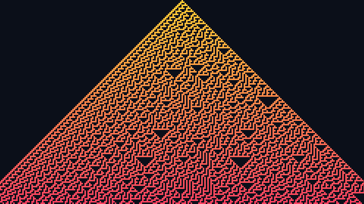
00011110Rule 30 grows from a single cell into a pattern that looks completely random. It was used to generate random numbers in the software Mathematica.
Time goes down: each row is the generation after the row above it. The row wraps around, so the left neighbor of the first cell is the last cell.
Our Elementary Cellular Automaton tool draws all 256 rules much bigger, with your own colors, and lets you download the pictures.
Conway's Game of Life
The most famous cellular automaton of all was invented in 1970 by the British mathematician John Horton Conway, and became famous when Martin Gardner described it in his "Mathematical Games" column in the magazine Scientific American. Conway called it the Game of Life, or just Life.
Life is played on a flat grid of square cells, each one alive or dead, with the Moore neighborhood: each cell has 8 neighbors. Conway chose his rules carefully, after many experiments, so that patterns would be hard to predict: they should neither die out quickly nor grow without limit too easily. There are only three rules:
- Birth - A dead cell with exactly 3 live neighbors becomes alive.
- Survival - A live cell with 2 or 3 live neighbors stays alive.
- Death - Every other live cell dies: with 0 or 1 neighbors, of loneliness, and with 4 or more, of overcrowding.
Birth
3 neighbors. A dead cell with exactly 3 live neighbors comes to life.
Survival
2 neighbors. A live cell with 2 or 3 live neighbors stays alive.
Loneliness
1 neighbor. A live cell with fewer than 2 live neighbors dies.
Overcrowding
4 neighbors. A live cell with more than 3 live neighbors dies.
Conway described Life as a zero-player game: you choose the starting cells, and then you just watch. In the shorthand used by fans of Life, these rules are written B3/S23: a cell is Born with 3 neighbors, and Survives with 2 or 3.
Try it: play the Game of Life
Click or tap the cells to bring them to life or kill them (with a mouse you can also drag to draw), then click Step to see the next generation, or Run to watch it go. With Show the next generation turned on, the cells that are about to die are drawn in red, and the cells that are about to be born have a green outline, so you can check the rules yourself before each step.
Generation: 0
Live cells: 5
This board wraps around: a glider that leaves on the right comes back on the left, and one that leaves at the bottom comes back at the top. For much bigger boards, colors, rule variants, the famous patterns and video downloads, use our Game of Life tool.
The zoo of the Game of Life
Fans of Life have been cataloging its patterns for more than 50 years, and they gave them names, like a zoo. Most patterns fall into a few families:
Block
Still life
Every live cell has 3 neighbors, and no dead cell has exactly 3, so nothing changes.
Beehive
Still life
Another pattern that never changes.
Blinker
Oscillator, period 2
gen 0
gen 1
gen 2
Flips between a horizontal and a vertical line, forever.
Glider
Spaceship, period 4
gen 0
gen 1
gen 2
gen 3
gen 4
After 4 generations it has the same shape, one cell further down and to the right.
- Still lifes - Patterns that never change, like the block, the beehive, the loaf and the boat. A random start usually ends up as a scattering of these.
- Oscillators - Patterns that go through a cycle of shapes and come back to the first one. The period is the number of generations of the cycle: 2 for the blinker, the toad and the beacon, 3 for the pulsar, 15 for the pentadecathlon.
- Spaceships - Oscillators that come back to their first shape in a different place, so they travel across the grid. The glider, the smallest one, moves one cell diagonally every 4 generations. The lightweight, middleweight and heavyweight spaceships move sideways.
- Guns - Patterns that stay in place and shoot out spaceships forever. Conway first guessed that no pattern could grow forever, and offered a prize of 50 dollars to anyone who could prove him wrong. Bill Gosper won it in 1970 with the Gosper glider gun, which fires a new glider every 30 generations.
- Methuselahs - Tiny patterns that take a very long time to settle down. The R-pentomino, with only 5 cells (try it in the demo above), keeps changing for 1103 generations before it settles into 116 cells, including six gliders flying away. The diehard, with 7 cells, vanishes completely after exactly 130 generations.
All these patterns, including the Gosper glider gun, the pulsar, the acorn and the diehard, are ready to try in our Game of Life tool, and you can watch the same rules in three dimensions in our 3D Game of Life.
Other rules like Life
What happens if you change the numbers in B3/S23? Any choice of numbers of neighbors for birth (from 0 to 8) and for survival (from 0 to 8) gives a new automaton. These are called Life-like cellular automata, and there are 218 = 262,144 of them. Most are boring, but some have their own fascinating worlds:
| Name | Rule | What happens |
|---|---|---|
| Conway's Game of Life | B3/S23 | The original rule. Gliders, oscillators and glider guns. |
| HighLife | B36/S23 | Almost the same as Life, plus a replicator: a small pattern that makes copies of itself. |
| Seeds | B2/S | No cell ever survives. Every pattern explodes into a cloud of sparks. |
| Day & Night | B3678/S34678 | Live cells on a dead background behave exactly like dead cells on a live background. |
| Life without death | B3/S012345678 | Cells never die, so patterns grow into ladders and mazes forever. |
| Maze | B3/S12345 | Grows a labyrinth of narrow corridors from a small random seed. |
| Replicator | B1357/S1357 | Every pattern copies itself again and again, into a fractal of copies. |
You can run all of these, and many more, in our Game of Life tool, or type your own B/S rule there.
More states, more dimensions, continuous values
The Game of Life and the elementary rules have only 2 states and look only at their closest neighbors. Relaxing these limits opens up a huge variety of automata. Here are some of the best known, with a tool to try each one:
- Brian's Brain and the Generations rules - Cells have extra "dying" states: a cell that dies doesn't turn off at once, but fades through one or more states during which it can't come back to life. In Brian's Brain, invented by Brian Silverman, a cell is born when exactly 2 neighbors are alive, and always dies after one generation, so the grid fills with sparks and little ships that fly in all directions. Try it in our Generations Cellular Automaton, and in 3D in our 3D Cellular Automata.
- Wireworld - Also by Brian Silverman, with 4 states: empty, wire, and the head and tail of an electron. Electrons run along the wires, and with the right wire shapes you can build logic gates, and even a working computer that shows prime numbers.
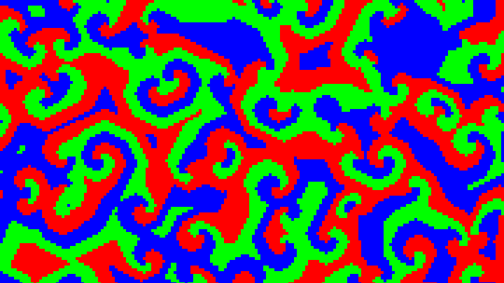
- The cyclic cellular automaton - Each cell has one of several colors arranged in a cycle, like red, then orange, then yellow, and back to red. A cell moves to the next color when enough of its neighbors already have it, like a game of "rock, paper, scissors". From random noise, the grid organizes itself into huge spirals. Try it in our Cyclic Cellular Automaton.
- The sandpile - Each cell holds a number of grains of sand. When a cell has 4 grains or more, it topples, giving one grain to each of its 4 neighbors, which may then topple in turn, in an avalanche. Pile up a million grains on one cell and they spread into an astonishing fractal. It was invented in 1987 by the physicists Per Bak, Chao Tang and Kurt Wiesenfeld to study avalanches and earthquakes. Try it in our Abelian Sandpile.
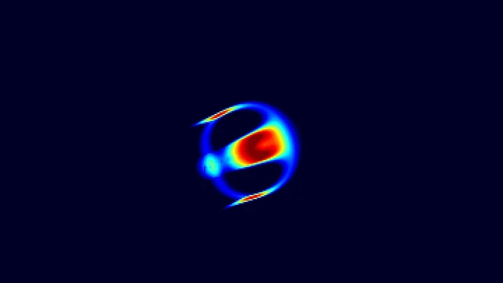
- Lenia - Created by Bert Wang-Chak Chan in 2018. Each cell holds any value between 0 and 1 instead of just 0 or 1, and looks at a large ring of neighbors, each with a different weight. With the right settings, it produces smooth "creatures" that glide, rotate and divide, and look strikingly like microscopic living things. Try it in our Lenia tool.
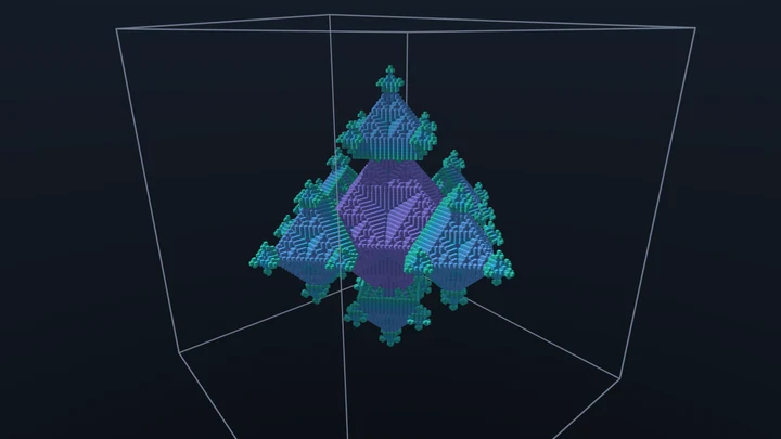
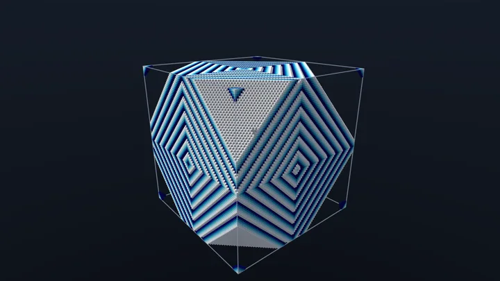
- 3D cellular automata - The same ideas work on a grid of cubes, where each cell has 26 neighbors in the Moore neighborhood. See our 3D Game of Life and 3D Cellular Automata.
How cellular automata are classified
Since each of the four ingredients can be changed, the natural way to classify cellular automata is by which ingredient they change: the grid, the states, the neighborhood or the rule. A completely different way, invented by Stephen Wolfram, is to ignore how they are built and look only at how they behave. The diagram below shows both. Click a group to jump to its explanation, or a "Try it" link to open the tool.
Cellular automaton
a grid of cells, a few states, a neighborhood, and one rule applied to every cell at once
Look at the behavior
- Class 1: uniform
- Class 2: stable or repeating
- Class 3: chaotic
- Class 4: complex
By the grid
- Number of dimensions - 1D automata live on a row, and are drawn as space-time diagrams. 2D automata live on a flat grid, and are drawn as an animation. 3D automata live in a block of cubes. Mathematicians also study automata in 4 or more dimensions, which can't be drawn directly.
- Shape of the cells - Square cells are the most common, but hexagonal cells, where every neighbor touches along a side, are popular for modeling nature, like the growth of snowflakes or the flow of fluids. Triangular grids exist too.
- What happens at the edges - A real computer can only hold a finite grid, so something must be decided at the border. The most common choice is to wrap around: the grid behaves as if its left edge were glued to its right edge and its top to its bottom, which turns it into the surface of a donut (a torus). The demos on this page work like that. Another choice is a fixed border, where all the cells outside the grid are dead. A third is a grid that grows when the pattern reaches its edge, which the best Life programs do, to imitate an endless grid.
By the states
- 2 states - Alive or dead, black or white: the elementary rules and the Game of Life.
- Several states - Like the dying states of Brian's Brain, the 4 states of Wireworld, or the colors of the cyclic automaton. Von Neumann's first self-copying automaton, from the 1940s, needed 29 states.
- Unlimited states - In the sandpile, a cell holds a number of grains, which can be as large as you want.
- Continuous states - Each cell holds any value in a range, like 0.37, as in Lenia. Strictly speaking these are no longer "classical" cellular automata, but they are built in the same way.
By the neighborhood
- von Neumann neighborhood - The 4 cells that share a side with the cell. Used by the sandpile and by von Neumann's self-copying automaton.
- Moore neighborhood - The 8 cells around the cell, diagonals included. Used by the Game of Life and most of its relatives.
- Larger neighborhoods - Cells can look further away: a 1D rule can look at 2 cells on each side instead of 1, and the "Larger than Life" rules count the live cells in a big square around each cell. Lenia uses a large ring of neighbors, with weights that fade with the distance.
By the rule
- General rules - The rule is a full table that gives the next state for every possible neighborhood, like the 8 boxes of the elementary rules. With 8 neighbors and 2 states there are 512 possible neighborhoods, and so 2512 possible rules, a number with 155 digits.
- Totalistic rules - The rule only depends on the sum of the states in the neighborhood, not on where each live cell is. A rule that also looks at the state of the cell itself, separately, is called outer totalistic: the Game of Life is one, since it only needs "how many neighbors are alive" and "is the cell alive". This is why Life-like rules can be written so briefly as B3/S23.
- Deterministic or probabilistic - In a deterministic automaton, the same neighborhood always gives the same result, so the same start always gives the same history. In a probabilistic (or stochastic) automaton, the rule rolls dice: for example, in the forest-fire model, a burning tree sets fire to its neighbors, but an empty cell grows a new tree only with some small probability.
- Synchronous or asynchronous - Classical automata update all the cells at the same time. Asynchronous automata update the cells one at a time, or in random order, which often gives very different results, and can be closer to how things happen in nature.
- Reversible - In a reversible automaton, every pattern has exactly one possible past, so the history can always be run backwards, like a movie in reverse. Most automata, including Life, are not reversible: many different patterns can end in the same pattern, so the past can't be recovered. Reversible automata are used to model physics, where the laws can run in both directions.
By the behavior: Wolfram's four classes
In 1984, Stephen Wolfram ran thousands of cellular automata from random starts and noticed that, whatever their rules, they always end up behaving in one of four ways. These Wolfram classes are the best known classification of cellular automata. The diagrams below show one elementary rule of each class, all started from the same random row of cells:
Class 1: uniform
Rule 160. Whatever the start, every cell soon becomes white, and nothing ever happens again.
Class 2: stable or repeating
Rule 108. The pattern quickly freezes into stripes, some fixed and some blinking every 2 steps.
Class 3: chaotic
Rule 30. The pattern never settles down, and looks random everywhere.
Class 4: complex
Rule 110. Structures that move and collide on a regular background, neither fixed nor random.
- Class 1 - Almost every start quickly becomes a uniform grid, all white or all black, and stays that way.
- Class 2 - The pattern quickly settles into a set of separate structures that are either fixed or repeat after a few steps. A change in one cell only affects a small area around it.
- Class 3 - The pattern stays chaotic forever and looks random. Changing a single cell at the start changes everything after a while, like the "butterfly effect" of the weather.
- Class 4 - Somewhere between order and chaos: structures that last a long time, move, and interact with each other in complicated ways. The Game of Life and Rule 110 are in this class, and it is the class where automata can compute, as we'll see below.
The classes are a description, not a precise mathematical definition, so some rules are hard to place, and some behave in one way from some starts and in another way from others. The computer scientist Chris Langton later suggested that class 4 lives at the edge of chaos: in the thin border between the rules that freeze and the rules that boil.
Close relatives
Some models look like cellular automata but break one of the rules. Their relationship is easiest to see by asking which things are discrete (made of separate steps, like cells and generations) and which are continuous (smooth, like real numbers):
| Model | Space | Time | States | Try it |
|---|---|---|---|---|
| Cellular automaton (Life, elementary rules) | Discrete: cells | Discrete: generations | Discrete: a few states | Game of Life |
| Lenia | Discrete on a computer, but designed so the cells can be made as fine as wanted | Discrete, with tiny steps | Continuous: any value from 0 to 1 | Lenia |
| Reaction-diffusion equations | Continuous | Continuous | Continuous: amounts of chemicals | Turing Pattern Generator |
| Turmites and Langton's ant | Discrete: cells | Discrete: steps | Discrete, but only one cell changes per step | Langton's Ant |
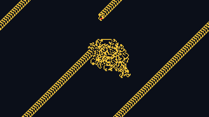
Langton's ant deserves a word. An "ant" walks on a grid of white cells: on a white cell it turns right, on a black cell it turns left, and in both cases it flips the color of the cell and moves forward. Unlike in a cellular automaton, only the cell under the ant changes at each step, so it is really a 2D Turing machine, called a turmite. Its behavior is famous: for about 10,000 steps it draws a chaotic blob, and then suddenly starts building a straight diagonal "highway" that repeats every 104 steps, forever. See it in our Langton's Ant and Turmite tools.
Many image filters are relatives too. A blur or an edge detection filter replaces every pixel by a combination of the pixels around it, with the same formula everywhere: that's exactly one step of a cellular automaton with continuous states. You can design your own in our Convolution Matrix tool.
Cellular automata that compute
A cellular automaton is called Turing complete, or universal, if it can imitate any computer program: with the right starting pattern, it can compute anything that any computer can compute (given enough cells and time). Amazingly, some very simple automata are universal:
- The Game of Life - Conway and his colleagues showed in 1982 that Life can compute anything. Streams of gliders work like electric signals, glider guns work like clocks, and gliders crashing into each other at the right angles work like the logic gates inside a computer chip. People have since built, out of Life patterns, a working Turing machine (Paul Rendell, in 2000), complete programmable computers, and even patterns that run the Game of Life itself, where each giant "metapixel" plays the role of one cell.
- Rule 110 - An elementary rule, with just 8 boxes, is also universal. Wolfram suspected it in 1985, and Matthew Cook proved it, in a proof published in 2004. It is one of the simplest universal systems ever found.
- Wireworld - Its wires carry electrons that work like the signals of real electronics, which makes building computers in it much easier than in Life.
This has a strange consequence. A famous result about Turing machines, the halting problem, says that no program can always predict whether another program will ever stop. Since Life can imitate any program, questions like "will this Life pattern ever die out?" or "will it grow forever?" are, in general, impossible to answer except by running the pattern and watching. Even with rules this simple, the future can't always be predicted. Read more in our article about Turing machines.
A short history
- 1940s - At the Los Alamos laboratory, the mathematician Stanislaw Ulam studies the growth of crystals using grids of cells, and his colleague John von Neumann wonders whether a machine could build a copy of itself. Following Ulam's suggestion, von Neumann designs a cellular automaton with 29 states, containing a pattern that can make copies of itself. His work is published after his death, in 1966.
- 1969 - The German computer pioneer Konrad Zuse suggests, in his book Calculating Space, that the universe itself might be a giant cellular automaton.
- 1970 - John Conway invents the Game of Life, published by Martin Gardner in Scientific American. Thousands of people start running it on the computers of their universities and offices. The same year, Bill Gosper finds the glider gun.
- 1983-1984 - Stephen Wolfram publishes his studies of the elementary cellular automata, with their numbering from 0 to 255 and his four classes of behavior.
- 1984-1986 - Christopher Langton creates "Langton's loops", much simpler self-copying patterns than von Neumann's, and Langton's ant. He goes on to found the field of artificial life.
- 1987 - Bak, Tang and Wiesenfeld introduce the sandpile model, and Brian Silverman invents Wireworld.
- 2002 - Wolfram publishes A New Kind of Science, a book of more than 1,200 pages arguing that simple programs like cellular automata can explain much of nature.
- 2004 - Matthew Cook's proof that Rule 110 is universal is published.
- 2018 - Bert Wang-Chak Chan presents Lenia and its lifelike creatures.
- 2020 - Researchers at Google present neural cellular automata, whose rule is a small neural network trained so that a single cell grows into a chosen image, like a lizard, and even regrows it when part of it is cut off.
What cellular automata are used for
Cellular automata are not just pretty pictures. Because they are built from local rules, like most things in nature, they are a natural way to model systems made of many simple parts:
- Nature - Forest fires spreading from tree to tree, epidemics spreading from person to person, the growth of crystals and snowflakes, and the patterns on some seashells, like the cone snail Conus textile, whose shell looks remarkably like Rule 30.
- Physics - "Lattice gas" automata, where particles hop between the cells of a hexagonal grid and bounce off each other, can imitate the flow of water and air. Sandpiles are used to study avalanches.
- Traffic - Rule 184 is the simplest model of cars on a road, and richer automata, like the Nagel-Schreckenberg model, reproduce real traffic jams that appear out of nowhere.
- Video games - Many games generate their caves by filling a grid with random walls and then applying a few steps of a "majority" rule, where each cell becomes a wall when most of its neighbors are walls. "Falling sand" games simulate sand, water and fire with one cell per grain. Our Maze Generator and the Maze rule of the Game of Life tool grow labyrinths in a similar way.
- Computer science - Random number generators (Rule 30), research into encryption, and special computers designed to run cellular automata very fast, because every cell can be computed at the same time.
- Art - Generative art, patterns and textures, like those you can create with our cellular automata tools, including Huegene, where colors spread and slowly mutate.
Frequently asked questions
Why is it called a cellular automaton?
"Cellular" because it is made of cells, like the squares of a grid, and "automaton" because, once started, it runs by itself, following its rule. The plural is "cellular automata".
Is the Game of Life a game?
Not in the usual sense: there are no players, no goal and no winner. Conway called it a zero-player game, because the only choice you make is the starting pattern. After that, the rules decide everything.
Can a pattern in the Game of Life grow forever?
Yes. The Gosper glider gun, found in 1970, shoots a new glider every 30 generations, forever, so the number of live cells grows without limit. Other patterns, called puffers and breeders, leave trails behind them or even build new guns as they go.
Can a cellular automaton run backwards?
Only if it is reversible. In the Game of Life, many patterns have no possible past at all: they can only appear as a starting pattern. They are called Gardens of Eden, and the Garden of Eden theorem (Moore, 1962, and Myhill, 1963) says that they exist exactly when two different patterns can turn into the same one.
What is the difference between a cellular automaton and a Turing machine?
A Turing machine has a single head that changes one cell at a time, while in a cellular automaton every cell changes at every step, all at once. But the two can imitate each other, so universal automata like Life can compute exactly the same things as a Turing machine. See our article about Turing machines.
Is the universe a cellular automaton?
Some scientists, like Konrad Zuse, Edward Fredkin and Stephen Wolfram, have suggested that the laws of physics might work like a cellular automaton at a very small scale. It is an interesting idea, but there is no evidence for it so far, and most physicists don't think it's likely.
Further reading
- Cellular Automata, in the Stanford Encyclopedia of Philosophy.
- Cellular automaton and Elementary cellular automaton, on Wikipedia.
- LifeWiki, the encyclopedia of the Game of Life and its patterns.
- Growing Neural Cellular Automata, an interactive article about neural cellular automata.
Related tools