
SmoothLife
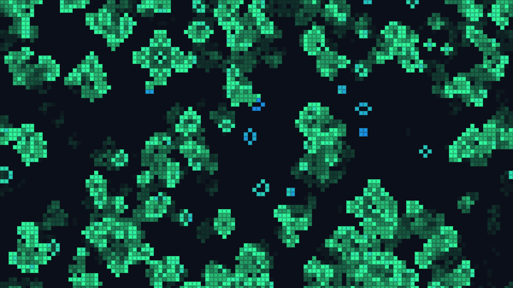
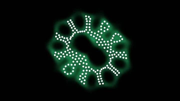
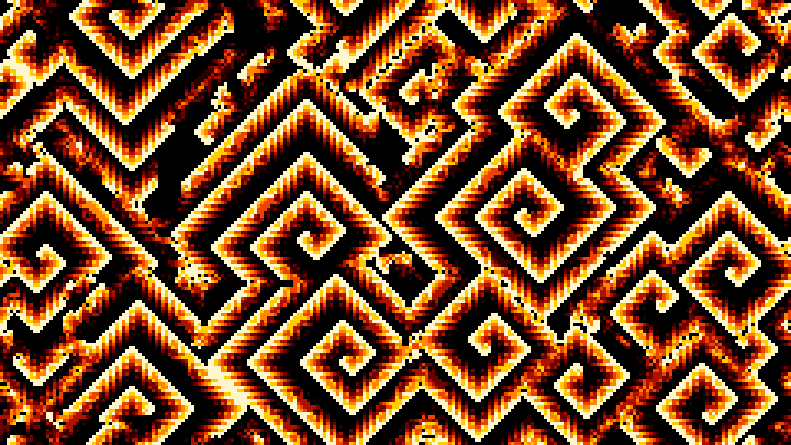
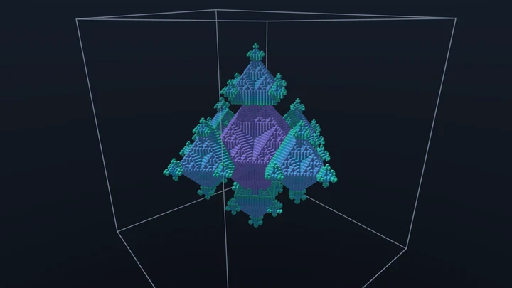
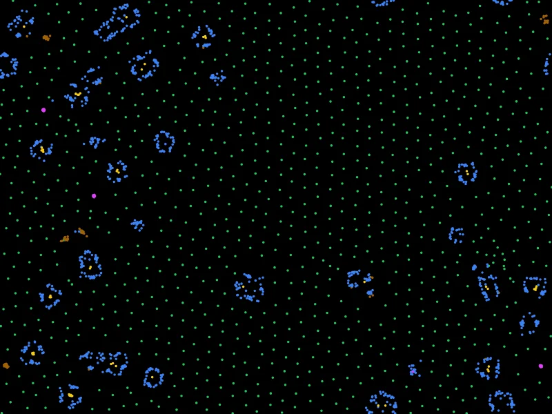
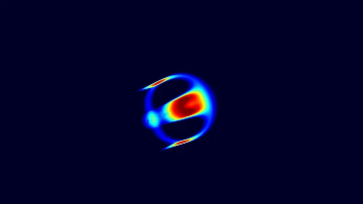
Watch smooth gliders, worms and oscillators emerge from SmoothLife, the continuous version of Conway's Game of Life created by Stephan Rafler. Choose one of the parameter sets of the original program, change the birth and death intervals while it runs, draw on the grid, and download images, GIFs and videos.
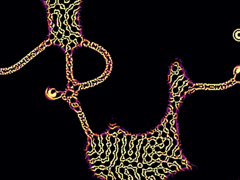
This is an online SmoothLife simulator. SmoothLife is the generalization of Conway's Game of Life to a continuous domain, published by Stephan Rafler in 2011. Instead of cells that are alive or dead, every point of the grid has a value between 0 and 1. Instead of counting 8 neighbors, every point measures how full a small disk around it is (the "cell") and how full the ring around that disk is (the "neighborhood"). The two numbers decide whether the point is born, survives or dies, through smooth versions of the birth and death rules of the Game of Life.
From this rule comes the smooth glider: a round creature that can fly in any direction, not only along the lines and diagonals of the grid like the gliders of the Game of Life. Many other forms of life appear with other parameters: worms, paragliders, blinkers, webs, honeycombs and rotating hexagons.
Choose one of the 26 parameter sets of the original program, switch between discrete and smooth time steps, change the radii, the birth and death intervals and the shape of the transition function while the simulation runs, and draw or erase on the grid with the mouse.
You can download the current state as a PNG image, or create an animated GIF or a WebM video. Everything runs directly in your browser: nothing is uploaded to a server. You are free to share the generated images and videos anywhere. Attribution is not required but appreciated.
Set: SmoothLifeLStep: 0Time: 0.0Filling: 0.00%Grid: 256 x 256
Click and drag on the grid to draw full disks.
Speed:
The parameter sets
Stephan Rafler shipped his SmoothLife program with a long list of parameter sets, each with a short name describing what he saw. The 26 sets below come from that list. Every one starts from random disks, like in the original program, with a seed where its structures appear: try other seeds to see how they vary. Click on any set to start it.
The smooth glider
ra = 12, discrete time, birth 0.278 to 0.365, death 0.267 to 0.445
The parameters of the original article, with discrete time steps: the generic smooth glider, a small round creature that can move in any direction, not only along the grid like the gliders of the Game of Life.
Paragliders and stable circles
ra = 12, discrete time, birth 0.362 to 0.47, death 0.258 to 0.554
Crescent shaped gliders, the paragliders, fly among circles that don't move. When a paraglider hits a circle, both can disappear.
Colorful worms
ra = 12, discrete time, birth 0.188 to 0.209, death 0.281 to 0.707
Worms that crawl head first, grow longer and bend, until the grid is full of them.
Crazy worms
ra = 12, discrete time, birth 0.216 to 0.269, death 0.284 to 0.605
A restless tangle of worms and bubbles that never settles down.
The rule of Conway, made smooth
ra = 12, discrete time, birth 0.3125 to 0.4375, death 0.1875 to 0.4375
The birth and survival rule of the Game of Life (B3/S23), written as fillings: a cell is born with 2.5/8 to 3.5/8 of its ring filled, and survives with 1.5/8 to 3.5/8. The disks settle into small rings that hardly move.
Labyrinth
ra = 14.3, discrete time, birth 0.322 to 0.353, death 0.157 to 0.673
The disks grow into a labyrinth of stripes, which keeps flickering and slowly rearranges itself. Rafler called it simply "pattern".
Gliders that change direction
ra = 24.6, discrete time, birth 0.262 to 0.328, death 0.269 to 0.434
Large gliders, with a radius twice as large, that turn from time to time in a random new direction.
SmoothLifeL
ra = 10, smooth time, dt = 0.1, birth 0.257 to 0.336, death 0.365 to 0.549
The parameter set of the famous SmoothLife video, with smooth time steps: the chaos of the start breaks up, and smooth gliders escape from it and fly away, alone or in pairs.
A swarm of small gliders
ra = 10, smooth time, dt = 0.1, birth 0.219 to 0.283, death 0.299 to 0.508
Many small gliders come out of the start and keep flying in every direction, bouncing off each other or merging. Rafler called this set "N".
Gliders pulling chains
ra = 10, smooth time, dt = 0.1, birth 0.257 to 0.336, death 0.355 to 0.549
A close cousin of SmoothLifeL ("K"), where the gliders pull long chains of small cells behind them.
Honeycomb
ra = 10, smooth time, dt = 0.1, birth 0.279 to 0.397, death 0.428 to 0.628
The whole grid fills with a honeycomb of small round cells, with a few defects that wander through it. It uses the overshooting step ("M").
Stable structures
ra = 10, smooth time, dt = 0.1, birth 0.377 to 0.336, death 0.365 to 0.799
The disks merge into blobs of strange shapes, which then freeze and never change again. Note that b1 is larger than b2.
Stable web
ra = 12, smooth time, dt = 0.1, birth 0.241 to 0.327, death 0.358 to 0.49
The disks dissolve into a web of thin threads, which join at knots and slowly straighten, like a soap foam.
Randomly curving gliders
ra = 16.5, smooth time, dt = 0.1, birth 0.247 to 0.314, death 0.328 to 0.51
Gliders that never fly straight: their path keeps curving one way and then the other.
Gliders and blocks
ra = 20.7, smooth time, dt = 0.095, birth 0.269 to 0.298, death 0.188 to 0.373
Gliders with a striped body move among blocks that stay still, and sometimes break them or are stopped by them.
Blobs with three skins
ra = 49.8, smooth time, dt = 0.097, birth 0.285 to 0.301, death 0.367 to 0.666
Large blobs wrapped in three concentric skins, on a radius of almost 50 cells, that hold together in pairs.
Schlieren gliders
ra = 12, smooth time towards s, dt = 0.041, birth 0.27 to 0.569, death 0.585 to 0.69
Round gliders swim through a sea of half-filled points, which ripples around them like the schlieren in hot air.
Circling gliders
ra = 12, smooth time towards s, dt = 0.1, birth 0.264 to 0.291, death 0.275 to 0.486
A crowd of small gliders that run around in circles, collide, split and merge, and never die out.
Cytogenetic wavefronts
ra = 12, smooth time towards s, dt = 0.1, birth 0.278 to 0.371, death 0.376 to 0.444
A tissue of cells, like the ones seen under a microscope, spreads in waves and retreats again. This set was found by someone else than Rafler.
Rotating hexagonal structures
ra = 12, smooth time towards s, dt = 0.107, birth 0.265 to 0.577, death 0.614 to 0.818
Islands full of holes, arranged in hexagons, float on a rippling sea of half-filled points and slowly turn.
Biphasic wobblers
ra = 12, smooth time towards s, dt = 0.115, birth 0.166 to 0.173, death 0.101 to 0.226
Small creatures that wobble between two shapes as they travel. The interval has a bump in its middle, and the set was found by someone else than Rafler.
Self-avoiding gliders
ra = 27.5, smooth time towards s, dt = 0.1, birth 0.212 to 0.244, death 0.222 to 0.397
Big gliders that seem to avoid each other, on a large grid.
Fishies
ra = 27.5, smooth time towards s, dt = 0.1, birth 0.218 to 0.248, death 0.225 to 0.328
A school of little fish, with a head and a body, that swim around the large grid.
Very smooth cone gliders
ra = 28.4, smooth time towards s, dt = 0.078, birth 0.195 to 0.25, death 0.219 to 0.509
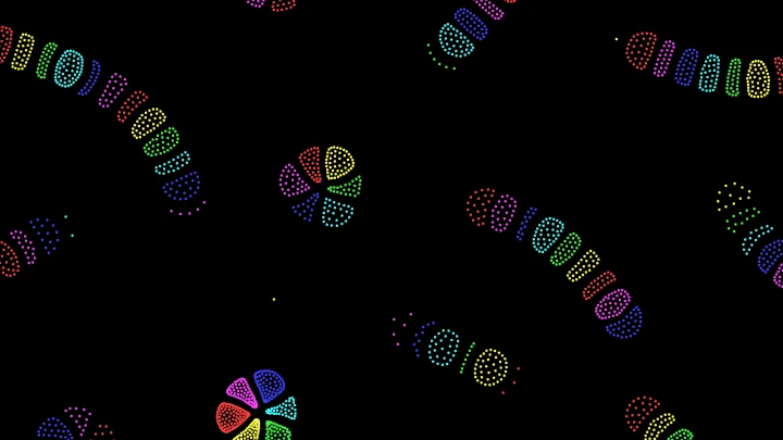
Long, very smooth gliders shaped like cones or worms, that move with their round head first.
Big blinkers
ra = 60.3, smooth time towards s, dt = 0.093, birth 0.184 to 0.209, death 0.284 to 0.585
Huge shapes with a radius of 60 cells, with rings and blobs that blink and wander.
Branching and nets
ra = 12, smooth time towards s, dt = 0.1, birth 0.235 to 0.292, death 0.563 to 0.9
A net of small cells grows out of the start, then branches and breaks into strands that drift away.
How to simulate SmoothLife
- Choose a parameter set - Keep SmoothLifeL, the set of the famous SmoothLife video, or choose another one: the smooth glider of the article, paragliders, worms, honeycombs, rotating hexagons... Each set comes with its grid and a seed that shows it well.
- Watch the structures emerge - The simulation starts from random disks. The first steps are chaotic, then the gliders, worms and oscillators appear. Use the speed buttons under the grid to go faster.
- Experiment with the rule (optional) - Change the birth and death intervals, the step widths, the radii or the time steps while the simulation runs, and watch the map of the transition function change with them.
- Change the start (optional) - Start from more or fewer disks, from random noise or from an empty grid, and try other random seeds.
- Draw on the grid (optional) - Click and drag on the grid to draw full disks or to erase, and see how the structures react.
- Pick the colors - Choose a palette, and show the state of the points, the filling of their rings or disks, or the transition function.
- Download it - Save the current image as a PNG, or the next steps as an animated GIF or a WebM video.
What is SmoothLife?
SmoothLife was described by Stephan Rafler in 2011 in the article Generalization of Conway's "Game of Life" to a continuous domain - SmoothLife, and became famous through his videos of smooth gliders. It continues an older line of work: Larger than Life, by Kellie Evans, which gives the Game of Life a larger neighborhood, and RealLife, by Marcus Pivato, its limit when the neighborhood becomes infinitely large.
Rafler's idea is to give the cell itself a size. A point of SmoothLife is not alive or dead by itself: it is alive when the small disk around it is full, and dead when that disk is empty. Its neighbors are the ring around the disk. With an outer radius three times the inner radius, the ring is three cells wide, like the 3 x 3 neighborhood of the Game of Life. Rafler called the result the "generic" generalization of the Game of Life, and its glider the generic glider: it looks like both the glider and the spaceships of the Game of Life, and it can fly in any direction.
A close relative of SmoothLife is Lenia, the continuous cellular automaton of Bert Chan, whose creatures look like microscopic organisms.
How does SmoothLife work?
On every step, every point of the grid is updated at the same time:
- The two fillings - The point measures the average of the values in the disk of radius ri around it, the inner filling m, and in the ring from ri to ra, the outer filling n. Both are between 0 and 1. The borders of the disk and of the ring are smoothed over a width b (anti-aliasing), so that the square grid doesn't show in the shapes.
- The transition function - The two numbers give the new state s(n, m). A point whose disk is empty (m close to 0) is born when n is in the birth interval [b1, b2]; a point whose disk is full (m close to 1) survives when n is in the death interval [d1, d2]. In the article, the borders of the intervals are smooth logistic steps of width αn, and the switch between the two intervals is a smooth step at m = 0.5, of width αm.
- The time step - With discrete time steps, the new value of the point is s(n, m). With smooth time steps, s(n, m) is turned into a speed of growth from -1 to 1, and the point changes by dt times that speed: f ← f + dt (2 s(n, m) - 1). The third mode of the original program moves the point a fraction dt of the way towards s(n, m): f ← f + dt (s(n, m) - f). The value is always kept between 0 and 1.
The transition function of the article is:
σ1(x, a) = 1 / (1 + exp(-4 (x - a) / α))
σ2(x, a, b) = σ1(x, a) (1 - σ1(x, b))
σm(x, y, m) = x (1 - σ1(m, 0.5)) + y σ1(m, 0.5)
s(n, m) = σ2(n, σm(b1, d1, m), σm(b2, d2, m))
σ2(x, a, b) = σ1(x, a) (1 - σ1(x, b))
σm(x, y, m) = x (1 - σ1(m, 0.5)) + y σ1(m, 0.5)
s(n, m) = σ2(n, σm(b1, d1, m), σm(b2, d2, m))
The disks and rings are computed with the fast Fourier transform, like in the original program, so the cost of a step doesn't depend on the radius: a ring of 60 cells is as fast as a ring of 10. That is why the sides of the grid are powers of two. The map next to the birth and death options draws s(n, m) for every n (from left to right) and m (from bottom to top): choose "The transition s(n, m)" in the "Show" option to see it applied to the grid.
The shapes of the transition function
The original program has more ways to build the transition function than the article, and many of its parameter sets use them:
| Option | Choices |
|---|---|
| Shape of the intervals | Moving interval (the article): one interval, whose borders move from [b1, b2] to [d1, d2] with the step in m. Two intervals, mixed by the step in m: the birth interval and the death interval are computed separately, and mixed by the step in m. Mixed linearly by m: the same, with m itself as the weight. Interval moving linearly with m: one interval, whose borders move linearly with m. |
| Shape of the steps in n and in m | The logistic function of the article, a hard step, a linear ramp, smoothstep (Hermite), a sine, the arctangent, the arctangent with a cosine wave, a logistic step that overshoots, and, for n only, logistic intervals with a dip or a bump in their middle. |
Options
Below are all the options you can configure in this SmoothLife simulator.
| Field | Description |
|---|---|
| Parameter set | One of the parameter sets of the original program. Choosing a set sets all the parameters of the rule, the size of the grid and the random seed, and starts the simulation again. |
| Time steps and time step (dt) | Discrete (the new value is s(n, m)), smooth (the value changes by dt (2 s(n, m) - 1)) or smooth towards s (the value moves a fraction dt of the way towards s(n, m)). The same rule gives different forms of life in each mode. |
| Outer radius (ra) | The outer radius of the ring, in cells. Larger radii give larger and smoother structures, and need a larger grid. |
| Ratio of the radii (ra / ri) | The outer radius divided by the radius of the disk. The usual value is 3, like the 3 x 3 neighborhood of the Game of Life. |
| Width of the smooth border (b) | The width, in cells, over which the borders of the disk and of the ring go from full to empty. 0 gives hard, jagged borders. |
| Birth (b1 to b2) and survival (d1 to d2) | The fillings n of the ring at which an empty point is born, and at which a full point survives. |
| Step widths (αn and αm) | How smooth the borders of the intervals are (αn), and how smooth the switch from the birth interval to the death interval is (αm). |
| Shapes of the intervals and of the steps | The other ways of building the transition function of the original program, described above. |
| Start with | Random full disks with a radius from ra/2 to ra (the start of the original program), random noise, or an empty grid to draw on. |
| Amount of disks, points with noise and random seed | How many disks are placed (1 is the amount of the original program), the percentage of points that get a random value, and the number that places them: the same seed always gives the same start. |
| Columns, rows and size of the cell | The size of the grid, from 64 to 1024 points on each side (powers of two, for the fast Fourier transform), and the size of each point in pixels. The edges of the grid wrap around. |
| Speed | The number of steps per second. "Maximum" computes as many steps as your computer can while keeping the page responsive. |
| Clicking on the grid and radius of the brush | Draw full disks or erase, with a brush of the given radius in cells. |
| Show | The state f of every point, the filling n of its ring, the filling m of its disk, or the transition s(n, m) it gets on the next step. |
| Palette and smooth pixels | The colors given to the values from 0 to 1, and whether the pixels are smoothed when the cells are enlarged. |
| Animation | The format (animated GIF or WebM video), the number of frames, the number of steps between two frames and the number of frames per second. The animation starts from the current state, with the size of the image. |
Frequently Asked Questions (FAQ)
Is this SmoothLife simulator free?Yes. The tool is completely free, there is no registration, and everything is computed by your own browser: nothing is uploaded to a server.
What is the difference between SmoothLife and the Game of Life?In the Game of Life, a cell is alive or dead, it counts its 8 neighbors, and the rule is a list of numbers of neighbors. In SmoothLife, every point has a value between 0 and 1, it measures the filling of a disk and of a ring around it, and the rule is two intervals of fillings. That is why the structures of SmoothLife look round and smooth, and why its gliders can move in any direction.
What is the difference between SmoothLife and Lenia?Both are continuous versions of the Game of Life. SmoothLife keeps the two numbers of the Game of Life, the state of the cell and the state of its neighbors, as the fillings of a disk and of a ring. Lenia, created later by Bert Chan, uses a single weighted ring and a growth function, and is known for its creatures that look like microorganisms.
Why did everything die, or fill the whole grid?Most parameter sets only live in a narrow range of parameters and starts. With a different seed, the disks may die out or merge into one big blob. Try another seed with the dice button, change the amount of disks, or choose the parameter set again to restore its parameters.
Why is the simulation slower with a large grid?Each step computes two fast Fourier transforms of the whole grid. A grid of 256 x 256 points takes a few milliseconds per step, a grid of 512 x 512 points about four times more, and a grid of 1024 x 1024 points about sixteen times more.
Can I download the animation as a video?Yes. In the "Download" section, choose "Animated GIF" or "Video (WebM)", the number of frames and the number of steps between two frames, and click on the download button. The animation starts from the current state of the grid.
Can I use the images and the videos commercially?Yes. The images and videos you generate are yours, and you can use them in any project.
Related tools