
Fractals
What a fractal is, why it can have a dimension like 1.585, how the Mandelbrot set and the other famous fractals are made, and how they are classified, explained from the beginning.
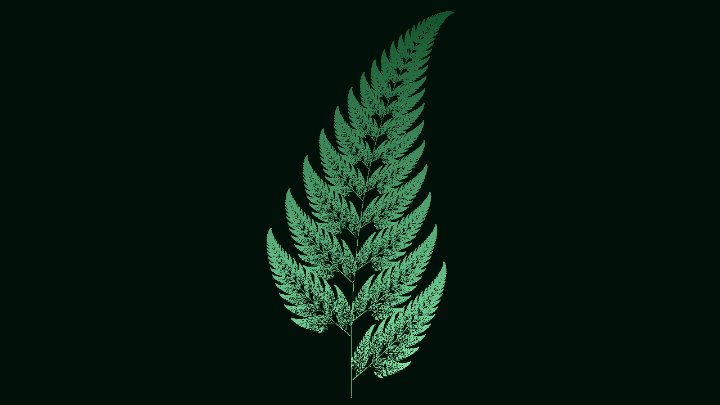
Look closely at a fern leaf: it is made of smaller leaves, and each of them looks like a small copy of the whole fern. Look at a stalk of broccoli, the branches of a tree or a map of a coastline, and you'll find the same trick: the shape is made of smaller copies of itself. Shapes like these are called fractals. Mathematicians have learned to build fractals with simple rules repeated again and again, and the results are some of the most beautiful and surprising pictures in all of mathematics: curves that are infinitely long but fit on a page, shapes with a dimension of 1.585, and a formula of a few symbols, the Mandelbrot set, that hides endless detail.
This article explains, without assuming any knowledge of advanced mathematics, what fractals are, how the famous ones are built, what their strange dimensions mean, and the many families of fractals, with diagrams that show how they are classified. You can grow fractals step by step, play the chaos game and explore the Mandelbrot set right on this page, and draw many more with our fractal tools.
Contents
- What is a fractal?
- Self-similarity: copies inside copies
- Building a fractal by repeating a rule
- Try it: grow a fractal
- An infinite border around a finite area
- How long is a coastline?
- Fractal dimension
- The chaos game
- The Mandelbrot set
- Try it: explore the Mandelbrot and Julia sets
- How fractals are classified
- Fractals in nature
- What fractals are used for
- A short history
- Frequently asked questions
What is a fractal?
A fractal is a shape that shows detail at every scale: however much you zoom in, you keep finding new structure, instead of the shape becoming smooth and simple. Most fractals are also self-similar: their small parts look like the whole.
Compare a fractal with an ordinary shape, like a circle. Zoom into the edge of a circle and it looks less and less curved; zoom enough and it looks like a straight line. Nothing new ever appears. Zoom into the edge of a fractal, and it stays just as wrinkled, branched or broken as before, however far you go. That's why the mathematician Benoit Mandelbrot, who invented the word in 1975, took it from the Latin fractus, which means "broken".
There isn't one precise definition of a fractal that every mathematician agrees on. In practice, a shape is called a fractal when it has most of these features:
- Fine detail at every scale - Zooming in never reveals a smooth, simple shape.
- Self-similarity - The parts look like the whole, exactly or roughly.
- A simple recipe - Despite the endless detail, the shape comes from a short rule repeated again and again.
- A strange dimension - The shape is too wrinkled to be a simple line, but too thin to fill an area, and its dimension is between the two, like 1.26 or 1.585.
Self-similarity: copies inside copies
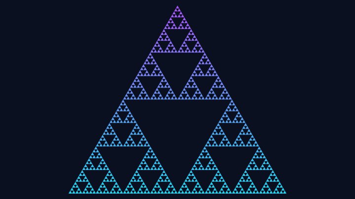
The easiest way to understand self-similarity is to zoom into a fractal. Below is the Sierpinski triangle, named after the Polish mathematician Wacław Sierpiński. Take its top corner and enlarge it 2 times: you get the whole triangle again. The same is true for the two bottom corners, and for the corners of the corners, forever.
Fractals differ in how exact their copies are, which gives a first way to classify them:
- Exact self-similarity - The parts are perfect, smaller copies of the whole, like in the Sierpinski triangle and the Koch curve. These fractals are built by geometric rules.
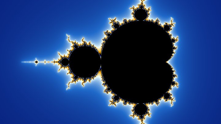
- Almost exact self-similarity (quasi-self-similarity) - The parts look like distorted copies of the whole. Zoom into the edge of the Mandelbrot set and you'll find many small copies of it, the "mini Mandelbrots", but each one is slightly twisted and surrounded by different decorations.
- Statistical self-similarity - The parts are not copies at all, but they are just as rough, or just as branched, as the whole. You can't tell how much you've zoomed. This is the kind of self-similarity found in nature: in coastlines, mountains, clouds and rivers.
Building a fractal by repeating a rule
Most famous fractals are built in the same way: start with a simple shape, apply a rule that replaces it by smaller pieces, then apply the same rule to every piece, again and again. Each round is called a step or an iteration. For the Sierpinski triangle, the rule is:
- Start with a filled triangle.
- Join the middles of its three sides, which cuts it into 4 smaller triangles, and remove the one in the middle.
- Do the same with each of the 3 triangles that are left, then with each of their 9 triangles, and so on.
Strictly speaking, the fractal is what you would get after an infinite number of steps. A computer, or a pencil, can only do a few, but after 6 or 7 steps the pieces are so small that the picture looks exactly like the true fractal.
Try it: grow a fractal
Pick a fractal, then add steps one at a time and watch how each step applies the same rule to every piece. The numbers on the right show what happens to the pieces, the length and the area as the steps go on.
Rule: Cut every triangle into 4 smaller triangles, and remove the one in the middle.
Step 3 of 7
| Triangles | 27 |
| Side of each triangle | 1/8 |
| Area left | 42.2% |
Draw it bigger, with your own colors, in our Sierpinski Triangle Generator.
Look at the numbers: they tell strange stories. The Sierpinski triangle loses a quarter of its area at every step, so after 10 steps less than 6% is left, and after infinitely many steps its area is zero, even though it still covers the whole triangle with its pattern. The Cantor set, the oldest of these fractals, published by Georg Cantor in 1883, ends up as a "dust" of infinitely many points with a total length of zero.
An infinite border around a finite area
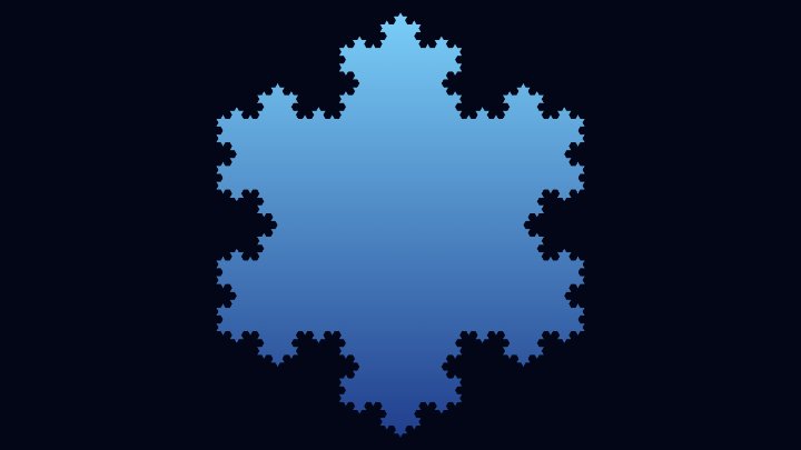
The Koch snowflake, described by the Swedish mathematician Helge von Koch in 1904, shows one of the most famous surprises of fractals. Start with a triangle whose sides have length 1. At every step, each segment of the border is cut into 3 thirds, and the middle third is replaced by two segments of the same length, which make a small spike. So every segment becomes 4 segments, each 1/3 as long, and the border gets 4/3 times longer at every step.
| Step | Segments | Perimeter | Area (the first triangle = 1) |
|---|---|---|---|
| 0 | 3 | 3.00 | 1.0000 |
| 1 | 12 | 4.00 | 1.3333 |
| 2 | 48 | 5.33 | 1.4815 |
| 3 | 192 | 7.11 | 1.5473 |
| 4 | 768 | 9.48 | 1.5766 |
| 5 | 3,072 | 12.64 | 1.5896 |
| 10 | 3,145,728 | 53.27 | 1.5998 |
| 20 | 3,298,534,883,328 | 946.01 | 1.6000 |
The perimeter keeps growing without limit: after 20 steps it is more than 300 times longer than at the start, and after infinitely many steps it is infinite. But the area hardly changes: each new spike is so small that the total area never goes above 1.6 times the area of the first triangle (exactly 8/5). The finished snowflake is a shape you could paint with a small pot of paint, but you could never walk all the way around it.
How long is a coastline?
This is not just a mathematical game. In the 1950s, the British scientist Lewis Fry Richardson was studying whether the length of the border between two countries had an effect on the chance of a war between them, and noticed something odd: different sources gave very different lengths for the same border. Spain said its border with Portugal was 987 km long, and Portugal said it was 1,214 km long.
The reason is the length of the ruler. Measure a coast with a ruler 100 km long, and you skip over every bay smaller than 100 km. Measure it with a 1 km ruler, and you follow the small bays and capes, and the coast gets longer. With a 1 meter ruler, you go around every rock, and it gets longer still. A coastline behaves like the Koch curve:
Mandelbrot took up Richardson's measurements in a famous article of 1967, How Long Is the Coast of Britain?, and his answer was surprising: it depends on the length of the ruler, and there is no single true length. This is called the coastline paradox. What does stay the same is how fast the length grows as the ruler gets shorter, and that rate is the key to measuring fractals, as we'll see now.
Fractal dimension
We usually say that a line has 1 dimension (it only has a length), a flat square has 2 (length and width) and a cube has 3. There's a simple way to see this number. Cut a shape into copies half its size and count them:
A line is made of 2 half-size copies, a square of 4, and a cube of 8. These are 21, 22 and 23: the power is the dimension. Now try the same with the Sierpinski triangle: it is made of 3 half-size copies. So its dimension is the power of 2 that gives 3, which is about 1.585 (because 21.585 ≈ 3). It is more than a line, but less than a filled area.
The same works with any shrinking factor. In general, if a shape is made of N copies, each 1/s of its size, then N = sD, where D is the dimension. With logarithms, which a calculator computes with the "log" key: D = log(N) / log(s). For the Koch curve, made of 4 copies 1/3 as big, D = log(4) / log(3) ≈ 1.262. This number, called the similarity dimension, is a simple case of the fractal dimension.
| Fractal | Made of | Dimension | Try it |
|---|---|---|---|
| Cantor set | 2 copies, 1/3 the size | 0.631 | |
| Koch curve | 4 copies, 1/3 the size | 1.262 | Koch Snowflake Generator |
| Sierpinski triangle | 3 copies, 1/2 the size | 1.585 | Sierpinski Triangle Generator |
| Sierpinski carpet | 8 copies, 1/3 the size | 1.893 | |
| Dragon curve | 2 copies, 1/√2 the size | 2 | Dragon Curve Generator |
| Menger sponge | 20 copies, 1/3 the size | 2.727 |
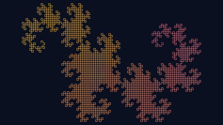
The dragon curve is a surprise: it's a line, but it bends so much that its dimension is exactly 2, the dimension of an area, and enough copies of it fill the plane. Other fractals have dimensions that can't be found by counting copies, and are measured instead: the most common method, called box counting, covers the shape with a grid of squares and counts how many squares touch it, for smaller and smaller squares. With this kind of measurement, the west coast of Britain has a dimension of about 1.25, and the border of the Mandelbrot set was proven by Mitsuhiro Shishikura, in 1991, to have a dimension of exactly 2.
The dimension says how rough a shape is, or how much it fills space. A curve with dimension 1.0 is smooth; at 1.25 it is wiggly like a coastline; close to 2 it is so crumpled that it almost fills an area. For the coastline paradox, the dimension tells how fast the length grows: with a ruler s times shorter, a coastline of dimension D looks about sD-1 times longer.
The chaos game
Here is a game that looks like it should produce a random mess. Mark the 3 corners of a triangle and put a point anywhere. Then, again and again:
- Choose one of the 3 corners at random, as if rolling a die.
- Move the point halfway towards that corner, and draw a dot there.
Try it below. Press 1 jump a few times to see each move (the dashed line goes from the point to the chosen corner), then Run to make thousands of jumps.
Jump halfway to one of the 3 corners, chosen at random. Each point gets the color of the corner it jumped to, which shows the 3 half-size copies of the triangle.
Points: 0
Out of pure randomness, the Sierpinski triangle appears, every time. The reason is self-similarity: moving halfway towards a corner shrinks the whole picture to half its size, towards that corner, which is exactly how one of the 3 copies of the Sierpinski triangle is made from the whole. Whatever the starting point, after a few jumps the point is so close to the triangle that the difference can't be seen, and the random jumps then visit every part of it. The colors show this: the points that jumped to the red corner make up the red copy, and so on.
The same idea works with any set of shrinking rules, called an iterated function system, or IFS. In 1988, the mathematician Michael Barnsley showed that just 4 rules, which shrink, turn and move the picture, draw a fern that looks like a real plant: the Barnsley fern, the last example above. Draw it with millions of points in our Barnsley Fern Generator, and play the chaos game with the triangle in our Sierpinski Triangle Generator.
The Mandelbrot set
The most famous fractal of all doesn't come from cutting shapes, but from a tiny formula repeated over and over:
z → z² + c
It means: start with z = 0, then square z and add a fixed number c, and repeat with the result. Let's first try it with ordinary numbers. For each c, we look at the list of values of z that it produces, called the orbit, and ask a single question: does it escape (grow forever) or not?
| c | Values of z | What happens | Result |
|---|---|---|---|
1 | 0, 1, 2, 5, 26, 677, 458330, ... | Explodes: the numbers grow faster and faster. | Escapes after 3 steps: outside |
0 | 0, 0, 0, 0, 0, 0, 0, ... | Stays at 0 forever. | Never escapes: inside |
-1 | 0, -1, 0, -1, 0, -1, 0, ... | Repeats 0, -1, 0, -1, forever. | Never escapes: inside |
-2 | 0, -2, 2, 2, 2, 2, 2, ... | Lands on 2 and stays there. | Never escapes: inside |
0.25 | 0, 0.25, 0.313, 0.348, 0.371, 0.388, 0.4, ... | Creeps towards 0.5, but never gets there. | Never escapes: inside |
0.3 | 0, 0.3, 0.39, 0.452, 0.504, 0.554, 0.607, ... | Creeps up slowly, then suddenly explodes. | Escapes after 12 steps: outside |
-1.5 | 0, -1.5, 0.75, -0.937, -0.621, -1.114, -0.258, ... | Jumps around without ever settling down, but never escapes. | Never escapes: inside |
As soon as z gets further than 2 from zero, it is sure to grow forever, so the computer can stop there and say "escapes". The values of c whose orbit never escapes form the Mandelbrot set. With ordinary numbers it is boring: just the numbers from -2 to 0.25. It becomes a fractal when c is a complex number.
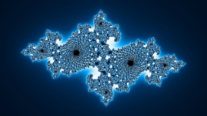
A complex number is a point on a flat plane, with two parts: a horizontal part (the "real" part) and a vertical part (the "imaginary" part, written with an i, like 0.3 + 0.5i). Complex numbers can be added and multiplied like ordinary numbers, with one extra rule, i × i = -1, and squaring a complex number has a simple meaning: it doubles its angle around zero and squares its distance from zero. Now every point of the plane is a possible c. For each one, the computer runs the formula, and colors the point black if its orbit never escapes. For the points that escape, the color shows how many steps it took. The result is the Mandelbrot set.
Its border is infinitely complex: zooming in reveals spirals, seahorses, lightning bolts, and small copies of the whole set, as deep as you want to go. Its area is about 1.506, but nobody knows a formula for it, and nobody has ever proved the exact number. The first rough pictures of it were printed in 1978 by Robert Brooks and Peter Matelski, and Mandelbrot studied it with the computers of IBM in 1980. Since then it has become one of the best known images of mathematics.
Julia sets
Julia sets use exactly the same formula, but the roles are swapped: c is fixed, and the starting value of z changes from point to point. For each point z of the plane, the computer runs the formula starting from that z, and colors it black if the orbit never escapes. Every value of c gives a different Julia set: there are infinitely many of them. They are named after the French mathematician Gaston Julia, who studied them with Pierre Fatou in 1918, more than 60 years before computers could draw them.
The two are deeply connected: the Mandelbrot set is a map of all the Julia sets. When c is inside the Mandelbrot set, its Julia set is all in one piece (mathematicians say it is connected). When c is outside, its Julia set breaks into infinitely many separate points, a "dust". And near its border, the Mandelbrot set around c often looks like the Julia set of c.
Try it: explore the Mandelbrot and Julia sets
Click or tap anywhere on the Mandelbrot set (left) to choose c. The white dots show the orbit of 0: the first values of z, joined by a line. The dashed circle has radius 2: once the orbit leaves it, it escapes. On the right is the Julia set of the same c. With a mouse, drag over the Mandelbrot set to watch the Julia set change continuously.
Mandelbrot set: choose c
Julia set of c
c = -0.123 + 0.745i
The orbit of 0 stays inside the circle (we checked 1,000 steps), so c is in the Mandelbrot set, and its Julia set is all in one piece.
Try the points near the edge of the Mandelbrot set: that's where the most interesting Julia sets are. Inside the big heart-shaped region (the main cardioid), the orbit spirals towards a single point; in the round bulb on its left, it ends up jumping between 2 points; in the smaller bulbs, between 3, 4, 5 or more. To zoom deep into these sets, use our Mandelbrot Set Generator and Julia Set Generator.
How fractals are classified
Fractals can be grouped in several ways: by their dimension, by how exact their self-similarity is, or, most often, by how they are made. The diagram below groups the best known fractals by the method used to build them. Click a group to jump to its explanation, or a "Try it" link to open the tool.
Fractal
a shape with detail at every scale, usually made of smaller copies of itself
Add randomness
- Plasma and fractal terrainTry it
- Random walks
- Growth by sticking particles
How exact the copies are
- Exact: Sierpinski, Koch
- Almost: Mandelbrot, Julia
- Statistical: coastlines, clouds
Shrink and copy: iterated function systems
These fractals are made of a few smaller copies of themselves, each one shrunk, and maybe turned or moved. The Cantor set is made of 2 copies at 1/3 of the size, the Sierpinski triangle of 3 copies at 1/2, the Sierpinski carpet of 8 copies at 1/3, and its 3D version, the Menger sponge (Karl Menger, 1926), a cube with tunnels at every scale, of 20 copies at 1/3. The rules that make the copies form an iterated function system, and in 1981 John Hutchinson proved that every such system defines exactly one shape, which can be drawn by repeating the rules on any starting picture, or by playing the chaos game. The Barnsley fern belongs here too: it is 4 copies of itself, the leaflets and the stem.
Replace every piece: curves and L-systems
These fractals are drawn as lines, by replacing every segment with a small pattern of segments, again and again. The Koch curve replaces each segment by 4 segments with a spike, and the dragon curve, discovered in 1966 by the NASA physicists John Heighway, Bruce Banks and William Harter, is what you get when you fold a strip of paper in half again and again, and then open each fold to a right angle (see our Dragon Curve Generator). The Peano curve (1890) and the Hilbert curve (1891) are lines that twist so much that, in the end, they pass through every point of a square: they are called space-filling curves, and they have dimension 2.
In 1968, the biologist Aristid Lindenmayer invented a way to write such rules as text, now called L-systems, to model how plants grow. The Koch curve, for example, is the rule "F → F+F−−F+F": every "draw forward" (F) becomes four shorter ones, with turns of 60 degrees (+ and −) between them. With rules that also save and come back to a position, the same method grows remarkably realistic trees, bushes and flowers, like the fractal tree in the demo above. The drawing is done by a "turtle" that follows the commands, like in our Turtle Graphics tool.
Repeat a formula: escape-time fractals
These fractals color every point of the plane by running a formula from that point, and counting how many steps it takes to escape. The Mandelbrot set and the Julia sets use z → z² + c, as explained above. Small changes to the formula give whole new worlds:
- Higher powers - With z → z³ + c, z⁴ + c and so on, the "Multibrot" sets get 2, 3 or more lobes instead of one.
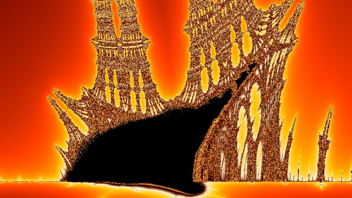
- The Burning Ship - Found by Michael Michelitsch and Otto Rössler in 1992. Before each squaring, the two parts of z are made positive, which breaks the smooth curves into sharp flames, and makes a shape that looks like a burning ship. See our Burning Ship Fractal Generator.
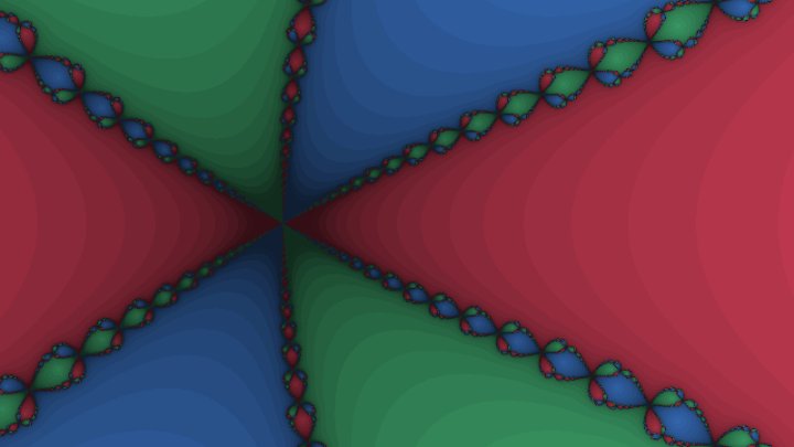
- The Newton fractal - Newton's method is a recipe for finding where an equation equals zero: start from a guess, and improve it again and again. For the equation z³ = 1 there are 3 answers, and the Newton fractal colors every starting point by the answer it ends up at. The borders between the colors are fractals, where all three colors meet everywhere. See our Newton Fractal Generator.
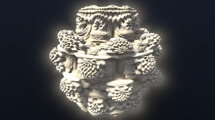
- The Mandelbulb - For a long time people looked for a 3D version of the Mandelbrot set. In 2009, Daniel White and Paul Nylander found a formula that works, using powers of points in 3D space, and called the result the Mandelbulb. Fly through it in our Mandelbulb 3D Fractal.
Add randomness: random fractals
Adding chance to the rules gives fractals with statistical self-similarity, which look much more like nature:
- Fractal terrain and plasma - Start with a square, and at each step, set the middle of each square to the average of its corners plus a random amount, with smaller and smaller random amounts at each step. This method, called midpoint displacement or diamond-square, makes landscapes that look like real mountains, and cloud and plasma textures. See our Plasma Fractal Generator.
- Random walks - The path of a particle that moves at random, like a speck of dust in water (Brownian motion), is a fractal: zoom into a part of the path and it looks just as tangled as the whole. In the plane, it has dimension 2.
- Growth by sticking particles - Let particles wander at random until they touch a growing cluster, and stick. The cluster grows into branching shapes like frost, coral or lightning, with a dimension of about 1.71. This model, called diffusion-limited aggregation, was introduced by Thomas Witten and Leonard Sander in 1981.
Simple rules, complex results
Fractals also appear by themselves, without anyone designing them, in systems that just follow simple rules:
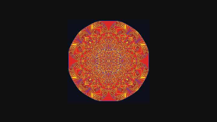
- Cellular automata - In a cellular automaton, a grid of cells changes step by step following a rule. The elementary rule called Rule 90, started from a single black cell, draws the Sierpinski triangle (see our Elementary Cellular Automaton), and the sandpile, where grains of sand topple onto their neighbors, piles up into an astonishing fractal (see our Abelian Sandpile). Read more in our article about cellular automata.
- Strange attractors - In chaos theory, the motion of systems like the weather can be drawn as a path in space. For chaotic systems, the path never repeats, but stays on a shape with fractal layers, called a strange attractor. The most famous, the Lorenz attractor (1963), looks like the wings of a butterfly, and has a dimension of about 2.06.
Close relatives: pictures inside pictures
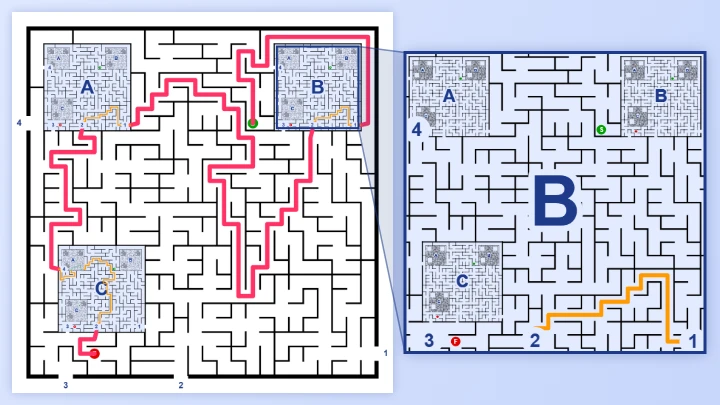
A picture that contains a smaller copy of itself, which contains a smaller copy, and so on, is called the Droste effect, after a Dutch cocoa box whose picture showed a nurse holding the same box. It is self-similar, but only around one point, so it isn't usually counted as a fractal. You can make your own in our Droste Effect Generator and Droste Spiral Generator, turn it into an endless zoom with the Infinite Zoom Animation Generator, or solve a maze that contains copies of itself in our Fractal Maze Generator.
Fractals in nature
Mandelbrot's most famous book, The Fractal Geometry of Nature (1982), begins with this observation: "Clouds are not spheres, mountains are not cones, coastlines are not circles, and bark is not smooth, nor does lightning travel in a straight line." Nature is full of fractal shapes, because growing by repeating the same simple process is the easiest way to build something large and complex:
- Plants - Ferns, trees and the cauliflower-like Romanesco broccoli, whose cones are made of smaller cones, arranged in spirals, which are made of even smaller cones.
- The body - The airways of the lungs branch again and again, about 23 times, to fit a huge surface for breathing inside the chest. Blood vessels and nerves branch in the same way, to reach every cell.
- Landscapes - Coastlines, mountain ranges, and rivers with their tributaries, which have tributaries of their own.
- Weather - Clouds, which look similar from a plane or from the ground, lightning bolts, and the branches of snowflakes.
Natural fractals are never infinite: the branching of a tree stops at the twigs, and the cones of a Romanesco stop after a few levels. They are self-similar only over a range of scales, which is still enough to make fractal geometry a much better description of them than circles and straight lines.
What fractals are used for
- Movies and video games - In 1980, Loren Carpenter showed a short film, Vol Libre, flying over mountains made of fractals, and was soon hired by Lucasfilm. Fractal landscapes appeared in the "Genesis" sequence of Star Trek II: The Wrath of Khan (1982), and fractal noise is still used today to create terrains, clouds, fire and textures, like the ones you can make with our Plasma Fractal Generator and Perlin Noise Generator.
- Antennas - An antenna shaped like a fractal curve packs a long wire into a small space, and can work at several frequencies at once, which makes it useful for small radios and phones.
- Image compression - Barnsley's idea that a complex picture can be described by a few shrinking rules led to fractal image compression, which stores an image as rules that copy parts of it onto other parts.
- Science and medicine - The fractal dimension is used as a measure of roughness: of coastlines, of surfaces of materials, of the branching of blood vessels in medical images, and of the shape of cells.
- Finance - Mandelbrot studied the prices of cotton in the 1960s and found that a chart of prices looks statistically the same over a day, a month or a year, an idea that changed how some economists think about risk.
- Art - Fractal art, made with programs that draw escape-time fractals and flames, is a whole field of digital art. Start with our fractal tools.
A short history
- 1872 - Karl Weierstrass describes a curve that is continuous, but has a sharp corner everywhere, so it is impossible to draw a tangent to it at any point. Many mathematicians call such shapes "monsters".
- 1883 - Georg Cantor publishes the Cantor set.
- 1890-1891 - Giuseppe Peano and David Hilbert describe curves that fill a whole square.
- 1904 - Helge von Koch describes the Koch curve, as an example of a curve without tangents that is easier to understand than Weierstrass's.
- 1915-1916 - Wacław Sierpiński describes the Sierpinski triangle and carpet.
- 1918 - Gaston Julia and Pierre Fatou study what happens when formulas like z² + c are repeated, and Felix Hausdorff defines a dimension that does not need to be a whole number.
- 1926 - Karl Menger describes the Menger sponge.
- 1967 - Benoit Mandelbrot publishes How Long Is the Coast of Britain?, and Martin Gardner makes the dragon curve famous in Scientific American.
- 1968 - Aristid Lindenmayer invents L-systems.
- 1975 - Mandelbrot coins the word "fractal".
- 1978-1980 - The first computer pictures of the Mandelbrot set.
- 1982 - Mandelbrot publishes The Fractal Geometry of Nature, and fractal mountains appear in Star Trek II.
- 1985 - A. K. Dewdney's column in Scientific American explains to its readers how to draw the Mandelbrot set on a home computer, and it becomes famous worldwide.
- 1988 - Michael Barnsley publishes Fractals Everywhere, with the Barnsley fern.
- 1991 - Mitsuhiro Shishikura proves that the border of the Mandelbrot set has dimension 2.
- 2009 - Daniel White and Paul Nylander find the Mandelbulb.
Frequently asked questions
Is a circle a fractal?
No. Zoom into the edge of a circle and it looks more and more like a straight line, so no new detail ever appears. Its dimension is exactly 1, like any smooth curve.
Are fractals infinite?
Their detail is infinite, but their size usually isn't: the Koch snowflake fits inside a circle, and the Mandelbrot set fits inside a circle of radius 2. What is infinite is the zoom: there is always more to see.
Why do the pictures of the Mandelbrot set have colors, if the set is black?
The set itself is only the black part. The colors around it are added to make it visible: each point outside is colored by the number of steps its orbit took to escape. Points just outside the border take many steps, which is why the colors show the shape of the border so clearly.
How far can you zoom into the Mandelbrot set?
Mathematically, forever. On a computer, ordinary numbers have about 16 digits, so the picture becomes blocky at a zoom of about 10 trillion (1013) times. Special programs use numbers with hundreds or thousands of digits to zoom much further, but they are much slower.
Can a fractal have a whole-number dimension?
Yes. The path of a random walk in the plane and the border of the Mandelbrot set both have dimension 2, although they are thin curves without any area. Mandelbrot's original definition said that a fractal is a shape whose fractal dimension is larger than its ordinary dimension, and these are curves (ordinary dimension 1) with a fractal dimension of 2. The dragon curve and the Hilbert curve also have dimension 2, but for a simpler reason: in the end, they fill a whole area. The border of the area filled by the dragon curve is itself a fractal, with a dimension of about 1.524.
Who invented fractals?
Many of the shapes were found between 1872 and 1926, by mathematicians like Cantor, Koch, Sierpiński and Julia, who saw them as curiosities. Benoit Mandelbrot gave them their name in 1975, showed with computers that they describe the shapes of nature, and found the Mandelbrot set's place at the center of the subject.
Further reading
- Fractal, Mandelbrot set and List of fractals by Hausdorff dimension, on Wikipedia.
- Coastline paradox, on Wikipedia.
- Fractals, a large collection of fractals with explanations and pictures, by Paul Bourke.
- The Fractal Geometry of Nature, by Benoit Mandelbrot (1982), and Fractals Everywhere, by Michael Barnsley (1988).
Related tools